Data Science for Business Applications

Class 01 - Linear Regression Review

What is Data Science?

• In Data Science we use the available data to obtain:

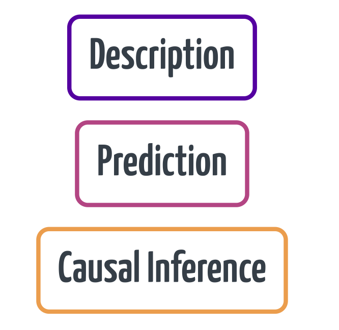
Data Science tasks

• Description: Can we classify our customers into different segments? (simple task)
• Prediction: What is the probability of a shopper coming back to our website? (kind of a simple task)
• Causal Inference: What is the effect of increasing our advertising budget on our total revenue? (difficult task)

Simple and Multiple Regression

• Linear Regression will be the most important tool for solving these Data Science tasks.
• Basically, in the linear regression model, we are explaining the relation between different variables by a line (that’s where the linear comes from.)
• Many fancy methods are generalizations or extensions of Linear Regression!
• In this class, we will do a quick review on linear regression.

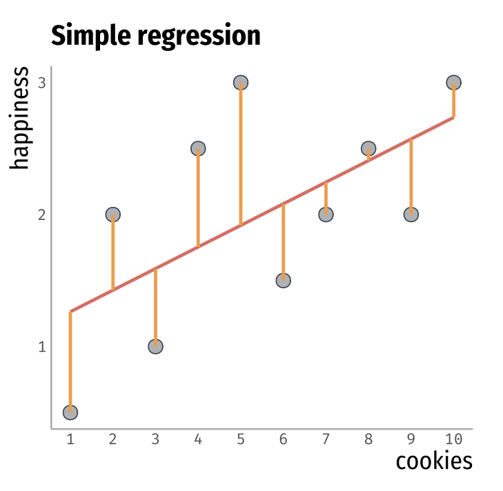
Cookie Example

• Suppose we have some data, and we want to understand how happiness changes in relation to the number of cookies eaten.
• To do so, we summarize the relation between these two variables through a line.
• This line is the linear regression line.
• Let’s see how this works!

cookies	happiness
1	0.1
2	2
3	1
4	2.5
5	3
6	1.3
7	1.9
8	2.4
9	1.8
10	3

Cookie Example

• The regression line is defined by two values, the intercept and the slope.
• The intercept is where the line intercepts the happiness axis.
• The slope relates to the inclination of the line.
• If the slope is positive the line has a upward direction.
• If the slope is negative the line has a downward direction.
• The regression line is a model of the relation between happiness and the number of cookies eaten.

Some questions on regression

• From the regression line, what is the relationship between happiness and the number of cookies eaten?
• Are there other factors other than the number of cookies that might affect the happiness level?
• From this model, can we conclude that eating cookies alone causes happiness?
• Why not look only at the correlation between happiness and the number of cookies?
• How do we obtain the intercept and the slope?
• Does this result apply to the entire population?

Regressions Details

• The Linear Regression model is represented by the formula: \[ Y = \beta_0 + \beta_1\cdot X_1 + \beta_2\cdot X_2 + e \]
• Multiple Regression means we have two or more \(X\)’s.
• Let’s break down this model into its essential parts.

Essential Parts of a Regression

• \(Y\) - Outcome Variable, Response Variable, Dependent Variable (Thing you want to explain or predict)
• \(X\) - Explanatory Variable, Predictor Variable, Independent Variable, Covariate (Thing you use to explain or predict \(Y\))
• \(\beta\)’s - Coefficients, Parameters (How \(Y\) changes numerically in relation to \(X\))
• \(e\) - Residual, Noise (Things we didn’t account in our model)

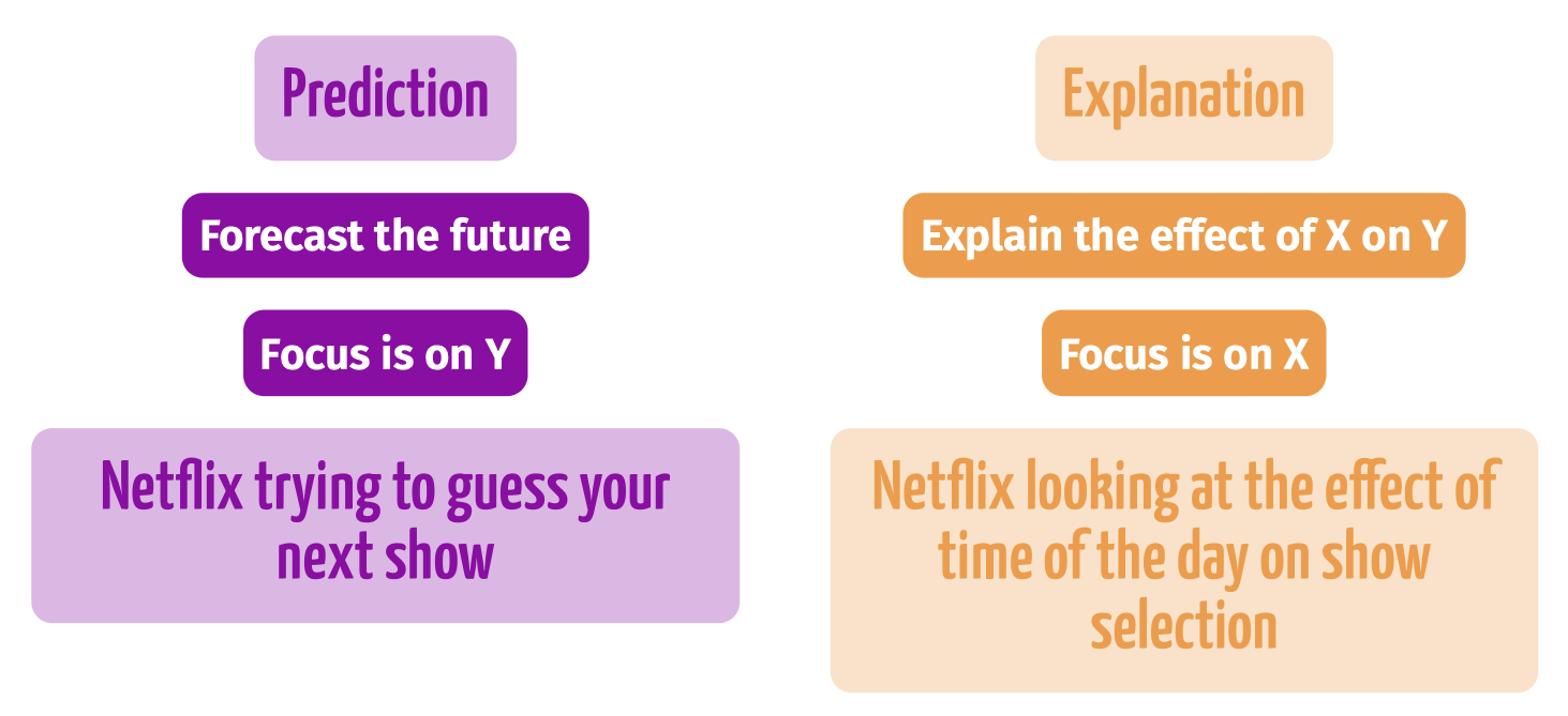
Two Purposes of Regression

Back to the Cookie example

• By writing the cookie example as a model where the variable happiness is the response variable and the number of cookies is the predictor, we have \[ \texttt{happiness} = \beta_0 + \beta_1\cdot\texttt{cookies} + e \]
• happiness is the response variable (\(Y\)).
• cookies is the predictor variable (\(X\)).
• \(\beta_0\) is the intercept.
• \(\beta_1\) is the slope associate to the cookies variable.
• \(e\) are the unknown factors that might explain the relation between cookies and happiness.
• The challenge now is to estimate the parameters \(\beta_0\), and \(\beta_1\).

How do we estimate the coefficients in a regression?

• A very useful strategy is use what is called the Ordinary Least Squares (OLS).
• The method is called ordinary least squares because the algorithm selects the coefficients (\(\beta\)’s) that minimize the sum of the squares of the errors in our sample.
• So the data in this case is fundamental.
• We use R to learn \(\beta\).
• The estimated coefficients are referred to as \(\widehat{\beta}\).

Let’s get into some data

• Example: Movie data Set (movie_1990_data.csv)
• We will create a model that explains and predicts the movie revenue in terms of the budget.
• There are 1,368 different movies in the data, with 22 different attributes.
• This means that the data contains 1,368 lines and 22 columns.
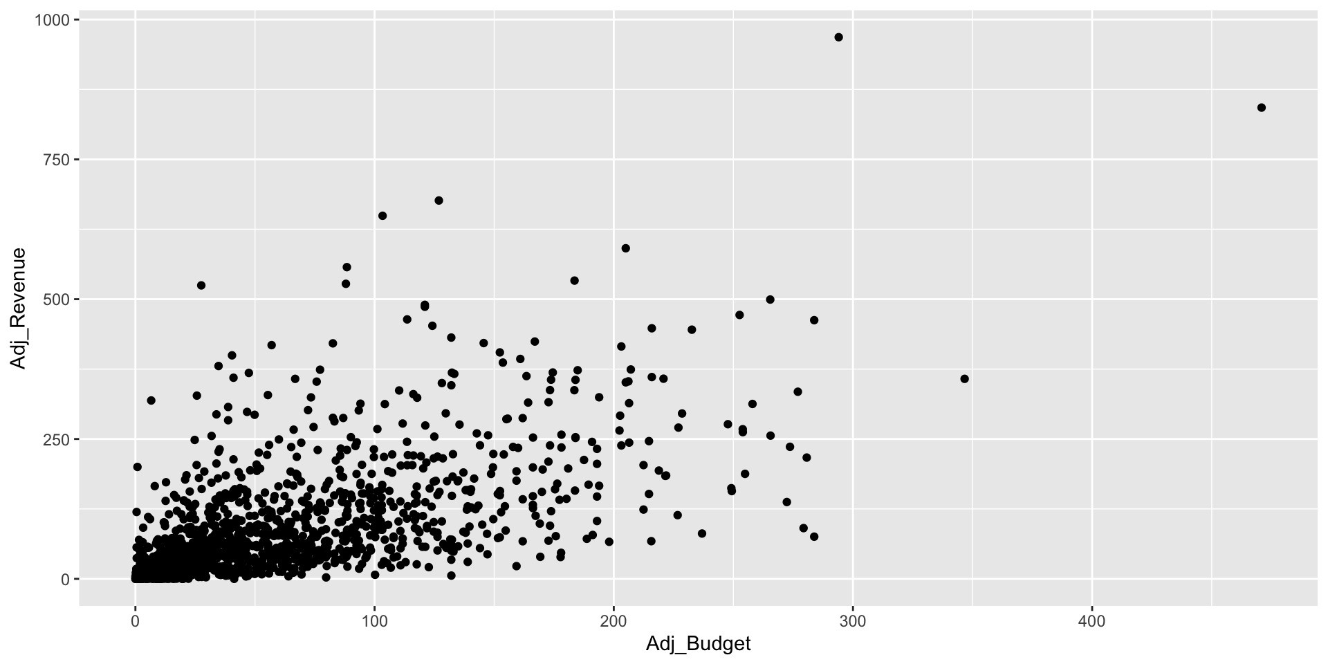
• We are interested in two attributes, the movie budget, and movie revenue.
• Movie budget is in the predictor variable - Adj_Budget.
• Movie revenue is in the response variable - Adj_Revenue.
• The units in this case are important (both are in millions of dollars).
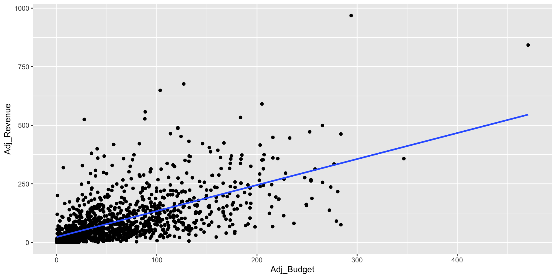
• Let’s visualize the relation between these two variables.

• First we load the library tidyverse, then we use the ggplot function to make plot between Adj_Budget and Adj_Revenue

# Load library
library(tidyverse)

# Create plot
ggplot(movie_1990_data) +
  geom_point(aes(x = Adj_Budget, y = Adj_Revenue))

We encode the model below in R.

\[ \texttt{Adj_Revenue} = \beta_0 + \beta_1\cdot\texttt{Adj_Budget} + e \]

# The model
# Revenue = intercept + slope*Budget + e
lm1 <- lm(Adj_Revenue ~ Adj_Budget, data = movie_1990_data)
summary(lm1)

Call:
lm(formula = Adj_Revenue ~ Adj_Budget, data = movie_1990_data)

Residuals:
    Min      1Q  Median      3Q     Max 
-262.40  -38.01  -16.39   19.24  619.23 

Coefficients:
            Estimate Std. Error t value Pr(>|t|)    
(Intercept) 22.66095    3.15001   7.194 1.03e-12 ***
Adj_Budget   1.11043    0.03738  29.709  < 2e-16 ***
---
Signif. codes:  0 '***' 0.001 '**' 0.01 '*' 0.05 '.' 0.1 ' ' 1

Residual standard error: 79.78 on 1366 degrees of freedom
Multiple R-squared:  0.3925,    Adjusted R-squared:  0.3921 
F-statistic: 882.6 on 1 and 1366 DF,  p-value: < 2.2e-16

Let’s interpret the output

• From the coefficients, \(\widehat\beta_0 = 22.7\), \(\widehat\beta_1 = 1.11\) we have the updated model: \[ \widehat{\texttt{Adj_Revenue}} = 22.7 + 1.11\cdot\texttt{Adj_Budget} \]
• When there’s a hat, it means that the values were generated from the data.
• \(e\) (noise) vanishes because we eliminated the unknown factors and concentrated the effect on what we observe.
• Now we have the residuals, that is the distance between the points in the data and the regression model.
• The question now is: how can we interpret this result?

Explanation

• Intercept: By setting the movie budget to zero, we have that the average revenue is equal to $22.7 million dollars.
• Slope: For one unit change in the movie budget, that is, millions, there will be an increase of $1.11 million dollars in the movie’s revenue.

Let’s visualize this model.

# Create plot with regression line
ggplot(movie_1990_data) +
  geom_point(aes(x = Adj_Budget, y = Adj_Revenue)) +
  geom_smooth(aes(x = Adj_Budget, y = Adj_Revenue), method = "lm", se = FALSE)

Statistical significance of the model

• Are these coefficients statistically significant?
• Can we extrapolate the results to the larger population?
• We can answer these questions by looking at the confidence interval (CI).

# We use the confint() function to get the confidence interval
confint(lm1)

                2.5 %    97.5 %
(Intercept) 16.481572 28.840332
Adj_Budget   1.037112  1.183756

Statistical significance of the model

From the confidence interval we have that:

• The value of the intercept is statistically different from zero since zero is not between the lower and upper values of the interval .
• The value of the slope is statistically different from zero since zero is not between the lower and upper values of the interval .

• With 95% confidence, the value of the intercept at the population level is between 16.5 and 28.8 million dollars .
• With 95% confidence, the value of the slope at the population level is between 1.04 and 28.8 million dollars .

Predictions

• Suppose we want to predict the revenue of a movie , knowing that the revenue was $25 million.
• We can use our estimated model to make the prediction.
• Input the value into the adjusted budget, resulting in: \[ \widehat{\texttt{Adj_Revenue}} = 22.7 + 1.11\cdot 25 = 50.45 \]
• The average predicted revenue of a $25 million dollar budget movie is $50 million dollars.
• We can also do this using the predict function in R

# We use the predict() function to get predictions
predict(lm1, list(Adj_Budget = 25))

       1 
50.42179 

Predictions

• How good are these predictions?
• We can use the residual standard error (RSE), which is a result of the summary function.
• \(\texttt{Residual standard error: 79.78}\),
• These mean that our predictions will be off by approximately 79.78.
• With 95% confidence, the prediction of the revenue will be 50.42 plus and minus \(2\times 79.78 = 159.56\).
• Quite a big variation.

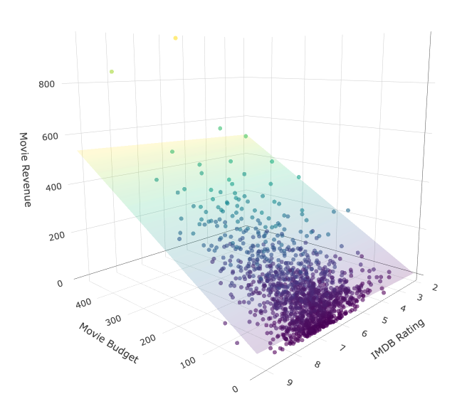
Adding more variables

• We can add more variables in our model.
• We will add the variable imdbRating which encodes the different IMDB ratings in the data (1-10).
• The resulting model now is \[ \texttt{Adj_Revenue} = \beta_0 + \beta_1\cdot\texttt{Adj_Budget} + \beta_2\cdot\texttt{imdbRating} + e \]
• You can observe that we have an extra slope in the equation.
• This will have an impact in how we interpret the model.
• Next we encode this model in R

Adding more variables

# The model
# Revenue = intercept + slope*Budget + slope*Rating + e
lm2 <- lm(Adj_Revenue ~ Adj_Budget + imdbRating, data = movie_1990_data)
summary(lm2)

Call:
lm(formula = Adj_Revenue ~ Adj_Budget + imdbRating, data = movie_1990_data)

Residuals:
    Min      1Q  Median      3Q     Max 
-256.79  -41.25  -14.97   26.55  598.53 

Coefficients:
              Estimate Std. Error t value Pr(>|t|)    
(Intercept) -136.50696   14.64962  -9.318   <2e-16 ***
Adj_Budget     1.09103    0.03585  30.433   <2e-16 ***
imdbRating    24.09935    2.17050  11.103   <2e-16 ***
---
Signif. codes:  0 '***' 0.001 '**' 0.01 '*' 0.05 '.' 0.1 ' ' 1

Residual standard error: 76.43 on 1365 degrees of freedom
Multiple R-squared:  0.4428,    Adjusted R-squared:  0.442 
F-statistic: 542.5 on 2 and 1365 DF,  p-value: < 2.2e-16

Visualizing the model

Explanation

• Let’s interpret the model:

\[ \texttt{Adj_Revenue} = -136.507 + 1.091 \cdot\texttt{Adj_Budget} + 24.099\cdot\texttt{imdbRating} \]

• Intercept: By setting the movie budget and the rating to zero, we have that the average revenue is equal to $-137 million dollars.
• Slope Budget: For movies with the same fixed rating, for one unit change in the movie budget, there will be an increase of $1.091 million dollars in the movie’s revenue.
• Slope Rating: For movies with the same fixed budget, for one unit change in the movie rating, there will be an increase of $24.1 million dollars in the movie’s revenue.

Statistical significance of the model

• Let’s analyse the confidence interval

# We use the confint() function to get the confidence interval
confint(lm2)

                  2.5 %      97.5 %
(Intercept) -165.245169 -107.768758
Adj_Budget     1.020706    1.161364
imdbRating    19.841475   28.357234

• All coefficients are statistically significant.

What about the predictions?

• We can observe from the summary that the residual standard error when down to \(\texttt{76.43}\).
• Which will result in more accurate predictions.
• Suppose we have a movie 25 million dollar budget and the movie has a IMDb rating of 5.4 what is the prediction for this movie?
• What about the 95% prediction interval for this prediction?

# We use the confint() function to get the confidence interval
predict(lm2, list(Adj_Budget = 25, imdbRating = 5.4))

       1 
20.90542 

• What about the 95% prediction interval for this prediction?
• upper bound: \(20.90542 + 2\times 76.43 = 173.7654\)
• lower bound: \(20.90542 - 2\times 76.43 = -131.9546\)

What’s next?

• We’ll include categorical variables.
• Interactions between categorical and numerical variables.