Data Science for Business Applications
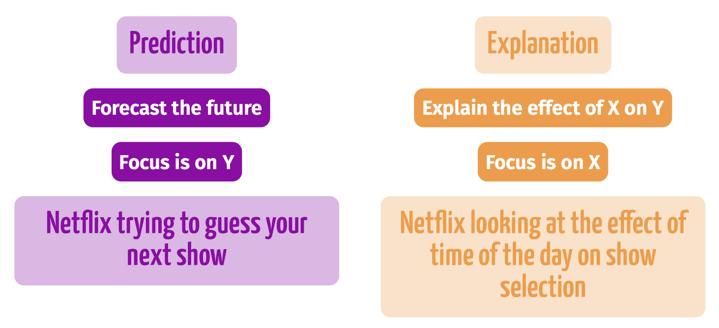
Regresison model goals
- Recall what are the goals of the linear regression model
Data Science tasks
- We found that adding more predictors to linear models increases their accuracy and explanatory power.
- What if we want to add instead of Quantative predictors, Qualitative predictors?
- Categorical or Qualitative Variables split the data into different groups or levels.
- How can we add these types of variables in the regression model?
Let’s start with an example!
- Example: Cars dataset (
cars_luxury.csv) - Data on 2,088 used cars in South California
- For each car there are several predictors as:
price: Price of the car in dollars.mileage: Car mileage.luxury: If the car is a luxury car: “\(\texttt{yes}\)”or “\(\texttt{no}\)”badge: Badge indicating if the car is considered some type of deal, that can be: “\(\texttt{Good Deal}\)”, “\(\texttt{Great Deal}\)”, “\(\texttt{No Badge}\)” or “\(\texttt{Fair Price}\)”.- (and others)
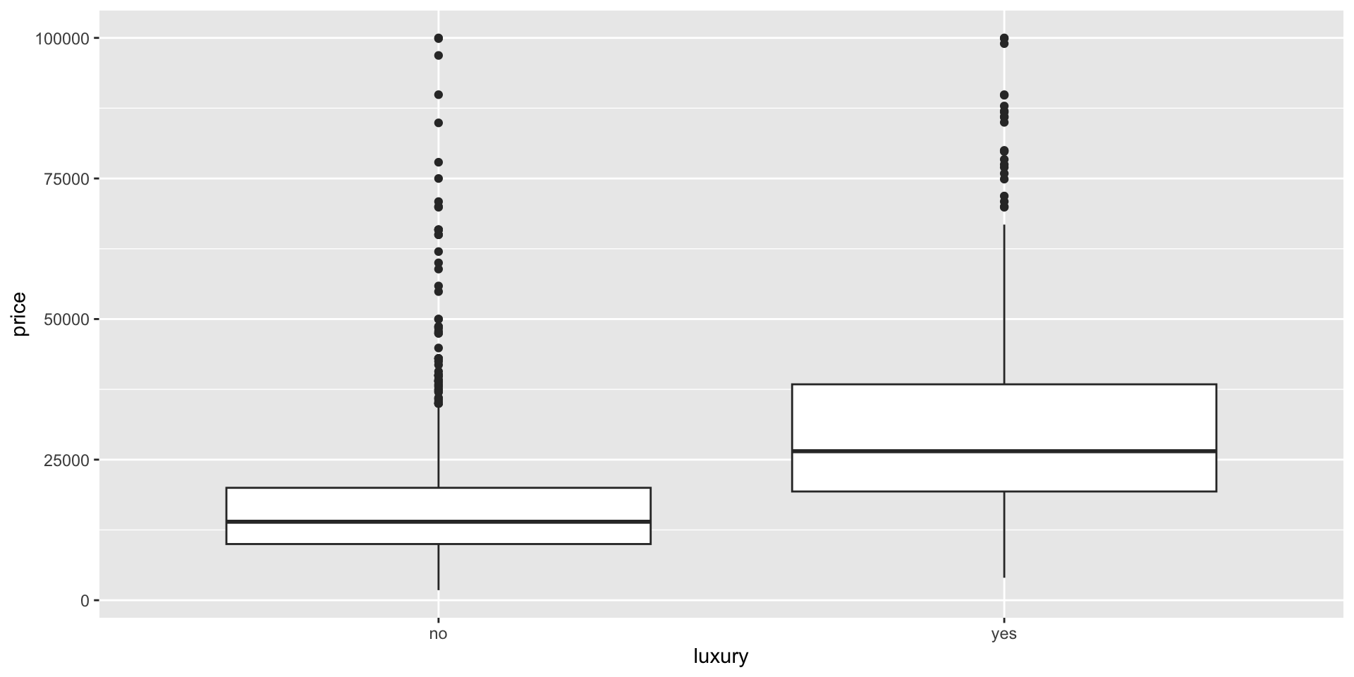
Luxury and price
- Before we start our analysis, let’s see if there’s a difference between the used price of luxury and not luxury cars.
Regression model
- It’s interesting to incorporate the categorical variable
luxury, into the multiple regression model. - We want to see the impact of mileage on price controlling for the type of car. If it’s a luxury or not.
- The resulting model is equal to: \[ \texttt{price} = \beta_0 + \beta_1\texttt{mileage} + \beta_2\texttt{luxury} + e \]
- How can we assess the categorical variable
luxury?
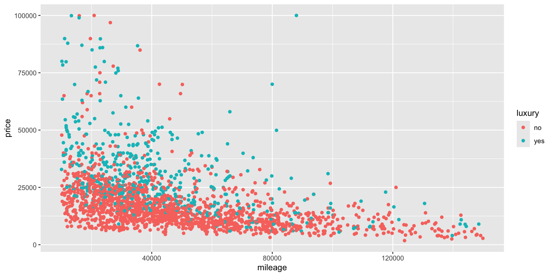
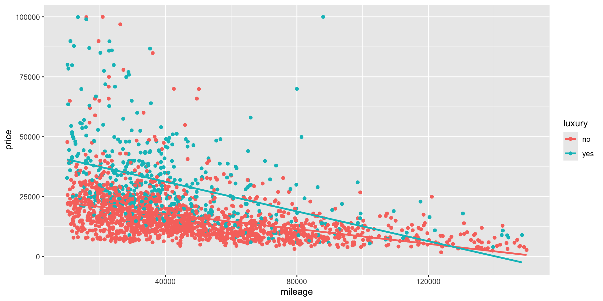
Price in terms of mileage and luxury
- Let’s plot the relation between
mileage,priceandluxury
Dummy variable
luxuryis a categorical variable (\(\texttt{"yes"}\) or \(\texttt{"no"}\) in this data set).- This variable contains two groups or two levels.
- Recode
luxuryinto a quantitative variable where \(\texttt{1 = "yes"}\), \(\texttt{0 = "no"}\). - This quantitative variable is known as dummy variable.
- R does this for us.
- R will choose the alphabetically first category as the 0 level.
Regression model
# Remove scientific notation
options(scipen = 999)

# Regression Model
lm1 = lm(price ~ mileage + luxury, data = cars_luxury)
summary(lm1)
Call:
lm(formula = price ~ mileage + luxury, data = cars_luxury)

Residuals:
   Min     1Q Median     3Q    Max
-24018  -6204  -1919   3727  78453

Coefficients:
                Estimate   Std. Error t value            Pr(>|t|)
(Intercept) 25422.756210   508.681485   49.98 <0.0000000000000002 ***
mileage        -0.185784     0.008688  -21.39 <0.0000000000000002 ***
luxuryyes   12986.388662   569.304402   22.81 <0.0000000000000002 ***
---
Signif. codes:  0 '***' 0.001 '**' 0.01 '*' 0.05 '.' 0.1 ' ' 1

Residual standard error: 11010 on 2085 degrees of freedom
Multiple R-squared:  0.3439,    Adjusted R-squared:  0.3433
F-statistic: 546.4 on 2 and 2085 DF, p-value: < 0.00000000000000022- How can we interpret these numbers?
Interpretation of the model
- Estimated model:
\[ \texttt{price} = 25,423 - 0.19\times \texttt{mileage} + 12,986 \times \texttt{luxury} \]
How can we interpret the coefficients?
intercept: For a car with zero mileage andluxury= \(\texttt{"no"}\) = 0, the average selling price is equal to US$ 25,423.mileage: For a fixed type of car, for each extra increase in mileage (in miles), there will be a decrease of US$ 0.19 in the price of the car.luxury: For cars with the same mileage, the added price of being a luxury car (luxury= \(\texttt{"yes"}\) = 1) is US$ 12,986.Important: When we add a categorical variable to the regression model, the intercept is also referred to as the baseline. The effect of the categorical variable is also known as the offset.
Interpretation of the model
By adding a categorical variable, we can also interpret this as different regression models depending on the number of groups.
To do so we add the effect of the categorical variable to the intercept.
luxury= \(\texttt{"yes"}\) = 1 \[ \begin{align} \texttt{price} &= 25,423 - 0.19\times \texttt{mileage} + 12,986 \times (1) \\ &= (25,423 + 12,986) - 0.19\times \texttt{mileage} \\ &= 38,409 - 0.19\times \texttt{mileage} \\ \end{align} \]luxury= \(\texttt{"no"}\) = 0 \[ \begin{align} \texttt{price} &= 25,423 - 0.19\times \texttt{mileage} + 12,986 \times (0) \\ &= 25,423 - 0.19\times \texttt{mileage} \\ \end{align} \]
Significance and Predictions
- Is the price of a luxury cars statistically different of a non-luxury car?
                    2.5 %        97.5 %
(Intercept) 24425.1797220 26420.3326977
mileage        -0.2028214    -0.1687463
luxuryyes   11869.9244244 14102.8528996
Yes, with 95% confidence we can conclude that the price of a luxury car is different from a non luxury one.
What is estimated price of luxury vehicle that has as mileage of 50000.
- The estimated price of a 50,000-mile luxury car will be US$ 29,120.
More than two groups
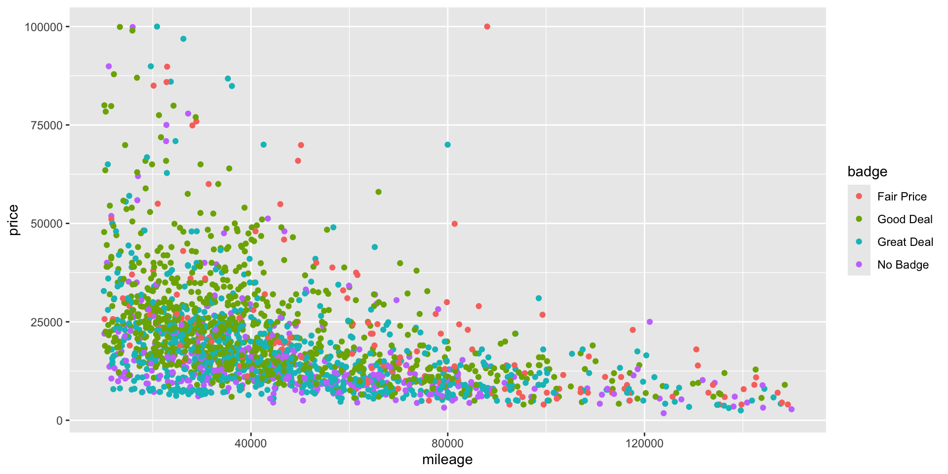
- Suppose, instead of controlling the fact that a car is a luxury car or not, we want to observe the effect of badge on price.
- The variable
badgecontains for groups or levels: “\(\texttt{Good Deal}\)”, “\(\texttt{Great Deal}\)”, “\(\texttt{No Badge}\)” or “\(\texttt{Fair Price}\)”. - Is there a difference in the price of the car depending on what type of badge it holds?
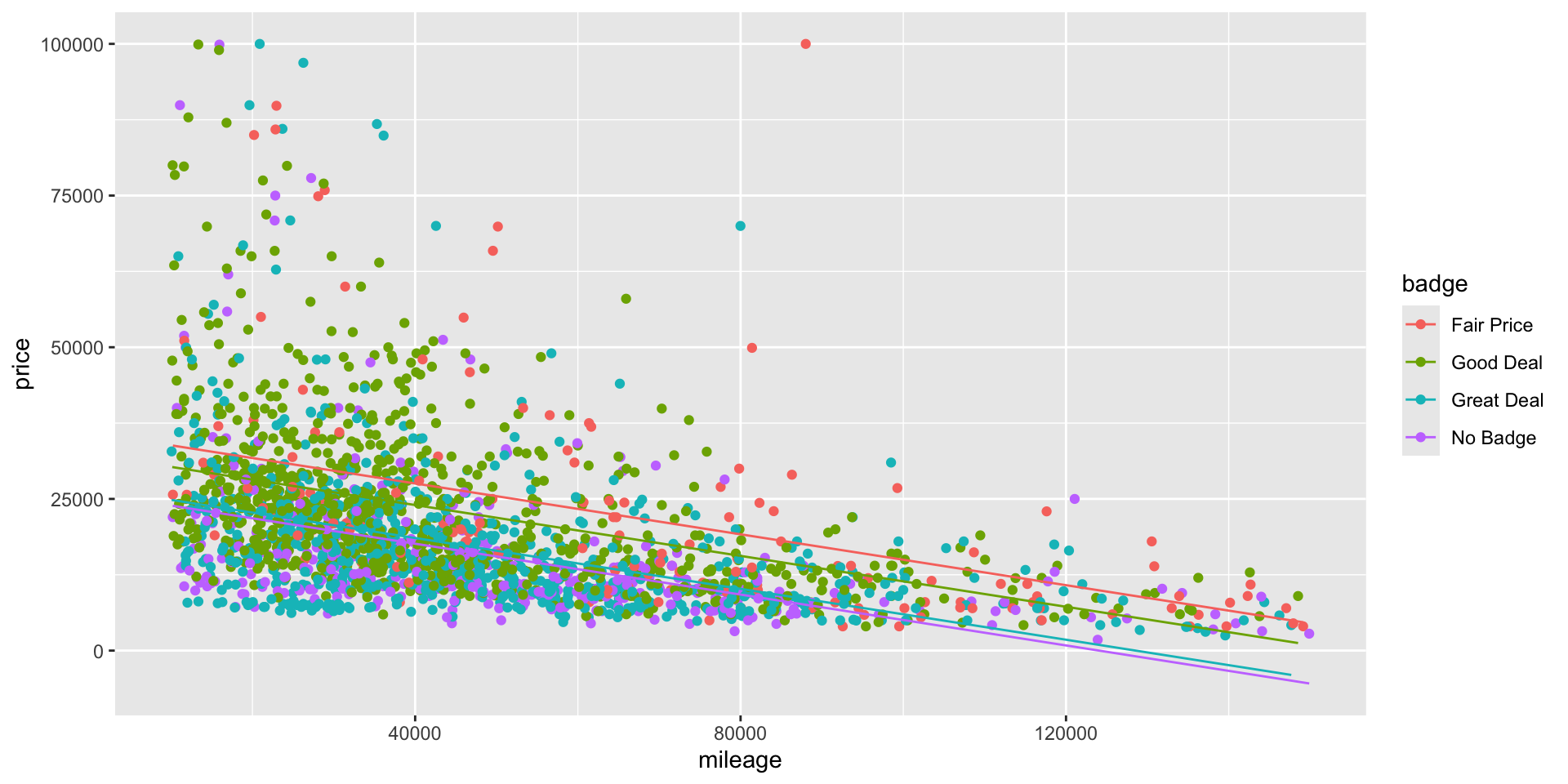
Regressions model
- Run the model: \(\texttt{price} = \beta_0 + \beta_1\times \texttt{mileage} + \beta_2 \times \texttt{badge} + e\)
Call:
lm(formula = price ~ mileage + badge, data = cars_luxury)

Residuals:
   Min     1Q Median     3Q    Max
-19961  -6981  -2395   3629  82508

Coefficients:
                    Estimate   Std. Error t value             Pr(>|t|)
(Intercept)     35931.481715  1140.032009  31.518 < 0.0000000000000002 ***
mileage            -0.209568     0.009527 -21.997 < 0.0000000000000002 ***
badgeGood Deal  -3556.561624  1057.385699  -3.364             0.000783 ***
badgeGreat Deal -8988.415770  1062.334934  -8.461 < 0.0000000000000002 ***
badgeNo Badge   -9930.896296  1143.713386  -8.683 < 0.0000000000000002 ***
---
Signif. codes:  0 '***' 0.001 '**' 0.01 '*' 0.05 '.' 0.1 ' ' 1

Residual standard error: 11860 on 2083 degrees of freedom
Multiple R-squared:  0.2388,    Adjusted R-squared:  0.2374
F-statistic: 163.4 on 4 and 2083 DF,  p-value: < 0.00000000000000022
Interpretation of the model
intercept(baseline): For a car with zero mileage and with a fair price badge, the average selling price is equal to US$ 35,932 (\(\texttt{Good Deal} = 0\),\(\texttt{Great Deal} = 0\), \(\texttt{No Badge} = 0\)).mileage: For a car with a fixed badge, for each extra increase in mileage (in miles), there will be a decrease of US$ 0.21 in the price of the car.\(\texttt{Good Deal} = 1\), remainig levels equal to zero: For cars with the same mileage, there will be a decrease in their price if they have a good deal badge of US$ 3,557 compared to the baseline, that is, cars with a fair price badge.
\(\texttt{Great Deal} = 1\), remainig levels equal to zero: For cars with the same mileage, there will be a decrease in their price if they have a great deal badge of US$ 8,988 compared to the baseline, that is, cars with a fair price badge.
\(\texttt{No Badge} = 1\), remainig levels equal to zero: For cars with the same mileage, there will be a decrease in their price if they have no badge of US$ 8,988 compared to the baseline, that is, cars with a fair price badge.
- We have now 4 different models, one for each badge catgory.
- We have four different intecepts.
Interactions
- We observed that there was a significant difference between the price of luxury and non-luxury cars.
- Is there a difference in the price of the car depending on what type of badge it holds?
- In other words, does the effect of one variable (i.e., its slope coefficient) depend on the value of another?
- For this we will include a interaction.
Interactions
- The idea is to add a term that is the product of the two variables:
\[ \texttt{price} = \beta_0 + \beta_1\texttt{mileage} + \beta_2\texttt{luxury} + \beta_3 (\texttt{luxury} \times \texttt{mileage}) + e \]
If we have a non-luxury car, then
luxury= \(\texttt{"no"} = 0\), so the \(\beta_2\) and \(\beta_3\) terms cancel out: \[ \texttt{price} = \beta_0 + \beta_1\texttt{mileage} + e \]If we have a luxury car, then
luxury= \(\texttt{"yes"} = 1\), so we get both a different intercept and a different slope for mileage: \[ \texttt{price} = (\beta_0 + \beta_2) + (\beta_1 + \beta_3) \texttt{mileage} + e \]
Regression Model
- Let’s run the regression model
Call:
lm(formula = price ~ mileage * luxury, data = cars_luxury)

Residuals:
   Min     1Q Median     3Q    Max
-25662  -6055  -2066   3563  83626

Coefficients:
                      Estimate   Std. Error t value             Pr(>|t|)
(Intercept)       23893.601384   545.040269  43.838 < 0.0000000000000002 ***
mileage              -0.154697     0.009595 -16.122 < 0.0000000000000002 ***
luxuryyes         19772.433662  1092.529243  18.098 < 0.0000000000000002 ***
mileage:luxuryyes    -0.155457     0.021457  -7.245    0.000000000000606 ***
---
Signif. codes:  0 '***' 0.001 '**' 0.01 '*' 0.05 '.' 0.1 ' ' 1

Residual standard error: 10880 on 2084 degrees of freedom
Multiple R-squared:   0.36, Adjusted R-squared:  0.3591
F-statistic: 390.8 on 3 and 2084 DF,  p-value: < 0.00000000000000022
Interpretation of the model
How do we interpret this model?
intercept(baseline),luxury= \(\texttt{"no"}\) = 0: For a non-luxury car with zero mileage, the average selling price is equal to US$ 23,894.Now we have two cases:
luxury= \(\texttt{"no"}\) = 0:mileage: For each extra increase in mileage (in miles), there will be a decrease of US$ 0.15 in the price of non-luxury cars.luxury= \(\texttt{"yes"}\) = 1:mileage: For each extra increase in mileage (in miles), there will be a decrease of US$ 0.16 in the price of luxury cars on top of the decrease of US$ 0.15 of non-luxury cars.
Interpretation of the model
We also have the following interpretation:
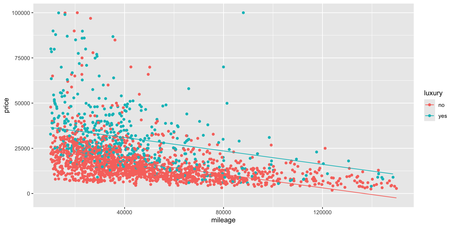
luxury= \(\texttt{"yes"}\) = 0 \[ \begin{align} \texttt{price} &= 23,894 - 0.15\times \texttt{mileage} + 19,772 (0) - 0.16\times \texttt{mileage} (0) \\ &= 23,894 - 0.15\times \texttt{mileage} \end{align} \]luxury= \(\texttt{"yes"}\) = 1 \[ \begin{align} \texttt{price} &= 23,894 - 0.15\times \texttt{mileage} + 19,772 (1) - 0.16\times \texttt{mileage} (1) \\ &= (23,894 + 19,772) - (0.15 + 0.16) \times \texttt{mileage} \\ &= 43,666 - 0.31 \times \texttt{mileage} \\ \end{align} \]We have that not only the intercept change but also the slope.
- The lines are not parallel in this case which indicates a change in the slope due to the intercation term.
Significance and Predictions
- Do luxury cars depreciate faster than non-luxury cars?
                          2.5 %        97.5 %
(Intercept)       22824.7212986 24962.4814687
mileage              -0.1735141    -0.1358795
luxuryyes         17629.8713295 21914.9959940
mileage:luxuryyes    -0.1975365    -0.1133770
Yes, with 95% confidence we can conclude that the price of a luxury car depreciates faster than a non-luxury one.
What is estimated price of luxury vehicle that has as mileage of 50000.
- The estimated price of a 50,000-mile luxury car will be US$ 28,158.
- There was also a decrese in the RSE of this model compared to the model without the interaction. From \(\texttt{11860}\) to \(\texttt{10,880}\).
Conlusion
- Interactions make a model more complex to analyze and explain, so it’s only worth doing so when you get better interpretation and more accurate predictions.
- We can have interactions between different kinds of variables. Between categorical variables, numerical and categorical and, numerical and numerical.
- Choose interactions by thinking about what you are trying to model: if you suspect that the impact of one variable depends on the value of another, try an interaction term between them
![]()