Data Science for Business Applications
Introduction to prediction
- So far, we have been focusing mostly on trying to explain the effects from the predictors \(X\) through the coefficients.
- Until now, our focus was on the soundness of our model in relation to statistical significance and how well our model was fitting the data (Regression Assumptions).
- Today, we will focus on making models that return Estimate/predict outcomes with high accuracy without extrapolating, with previously unseen data.
Inference and Prediction
Inference \(\rightarrow\) focus on the predictor
Interpretability of model
Prediction \(\rightarrow\) focus on outcome variable
Accuracy of model
Bias vs. Variance
Bias vs Variance trade-off
Variance: The amount by which the function \(f\) would change if we estimated it using a different training dataset
Bias: Error introduced by approximating a real-life problem with a model
More flexible models have a higher variance and a lower bias
Less flexible models have a lower variance but a higher bias
Validation set approach: Training and testing data
Balance between flexibility and accuracy
Bias vs. Variance
- When explaining, bias is usually greater than variance
- In prediction, we care about both
- Measures of accuracy will have both bias and variance
Measures of accuracy
How do we measure accuracy?
Mean Squared Error (MSE): Can be decomposed into variance and bias terms \[ \text{MSE} = \text{Var} + \text{Bias}^2 + \text{Irreducible Error} \] where MSE is equal to \[ MSE = \frac{1}{n} \sum_{i = 1}^n(y_i-\widehat{y}_i)^2 \]
Root Mean Squared Error (RMSE): Measured in the same units as the outcome \[ \text{RMSE} = \sqrt{\text{MSE}} \]
Other measures: Bayesian Information Criterion (BIC) and Akaike Information Criterion (AIC)
Is flexibility always better?
Measures of accuracy
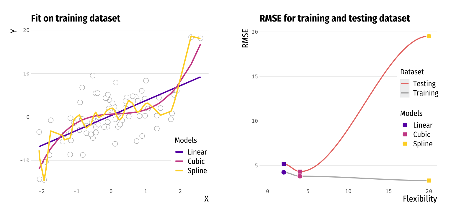
- Models with increasing flexibility (linear, cubic, spline).
- Think of a spline as a polynomial model with a high degree.
- RMSE decreases with flexibility in the training data.
- The spline overfits the training data since the RMSE of the testing data is large.
What is churn?
- Churn: Measure of how many customers stop using your product (e.g. cancel a subscription).
- Less costly to keep a customer than bring a new one
- Goal: Prevent churn
- Identify customer that are likely to cancel/quit/fail to renew

Predicting “pre-churn”
- We will predict “pre-churn”.
- At a good measure for someone at risk of unsubscribing (“pre-churn”) is the times they’ve logged in the past week.
- We are interested in the number of log ins in the variable
logins. - We will predict
loginsfrom the other variable in the data. - We two candidates: Simple vs Complex
Predicting “pre-churn”
Simple Model: \[ logins = \beta_0 + \beta_1 \cdot Succession + \beta_2 \cdot city + \epsilon \]
Complex Model: \[ logins = \beta_0 + \beta_1 \cdot Succession + \beta_2 \cdot age + \beta_3 \cdot age^2 + \beta_4 \cdot city + \beta_5 \cdot female + \epsilon \]
Can we build more complex methods? Yes!
First we will just analyse these two.
Create Validation Sets
- Create Training and Testing sets
- We will use 75% of the data to train the data
- The remaining part of the data, 25%, we reserve for testing
- This split is done randomly
- To do so we use the libraries
modelr, andrsample
RMSE in training and testing data
# Simple Model
lm_simple = lm(logins ~ succession + city, data = hbo_train)

# Complex Model
lm_complex = lm(logins ~ female + city + age + I(age^2) + succession, data = hbo_train)

# Testing error for the simple model:
rmse(lm_simple, hbo_test)
[1] 2.075106[1] 2.080211- Which model we should choose?
- The model with the smallest out of sample error
- Out of sample means evaluation in the testing data
Cross-Validation
- To avoid using only one training and testing dataset, we can iterate over k-fold division of our data:
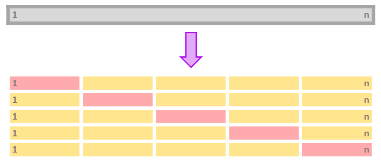
Grey: all of the data
Pink: Testing data
Yellow: Training data
Cross-Validation
Procedure for k-fold cross-validation:
Divide your data in k-folds (usually, \(K = 5\) or \(K = 10\)).
Use as \(k = 1\) the testing data and \(k = 2,3,\dots, K\) as the training data.
Calculate the accuracy measure on the testing data, \(RMSE_k\).
Repeat for each \(k\).
Average \(RMSE_k\) for all \(k\).
Main advantage: Use the entire dataset for training AND testing.
Apple quarterly revenue
- Install the library
caret
library(caret)
set.seed(100)
train.control = trainControl(method = "cv", number = 10)

lm_simple = train(logins ~ succession + city, data = hbomax, method= "lm", trControl = train.control)

lm_simple
Linear Regression
5000 samples
2 predictor
No pre-processing
Resampling: Cross-Validated (10 fold)
Summary of sample sizes: 4500, 4501, 4499, 4500, 4500, 4501, ...
Resampling results:
RMSE Rsquared MAE
2.087314 0.6724741 1.639618
Tuning parameter 'intercept' was held constant at a value of TRUEStepwise selection
We have seen how to choose between some given models. But what if we want to test all possible models?
Stepwise selection: Computationally-efficient algorithm to select a model based on the data we have (subset selection).
Algorithm for forward stepwise selection:
Start with the null model, (no predictors)
For : (a) Consider all models that augment with one additional predictor. (b) Choose the best among these models and call it .
Select the single best model from using CV.
- Backwards stepwise follows the same procedure, but starts with the full model.
Stepwise selection and CV
  nvmax     RMSE    Rsquared      MAE     RMSESD  RsquaredSD      MAESD
1     1 3.643876 0.001423859 3.168804 0.05856896 0.001837302 0.08173805
2     2 3.643778 0.002541723 3.168174 0.06094142 0.003036447 0.08474783
3     3 3.186594 0.206309738 2.719227 0.62445616 0.282844240 0.59591617
4     4 2.580810 0.468546464 2.125469 0.62430763 0.278310925 0.59607716
5 5 2.087951 0.672274342 1.640141 0.04906724 0.014296583 0.04888083- Which one would you choose out of the 5 models? Why?
- The model with the smallest RMSE, which is model 5.
- Can we see this model?
Stepwise selection and CV
- And how does that model looks like:
Subset selection object
6 Variables  (and intercept)
           Forced in Forced out
X              FALSE      FALSE
female         FALSE      FALSE
city           FALSE      FALSE
age            FALSE      FALSE
succession     FALSE      FALSE
id             FALSE      FALSE
1 subsets of each size up to 5
Selection Algorithm: forward
         X   id  female city age succession
1  ( 1 ) " " " " " "    " "  " " "*"
2  ( 1 ) " " " " " "    "*"  " " "*"
3  ( 1 ) " " " " " "    "*"  "*" "*"
4  ( 1 ) " " " " "*"    "*"  "*" "*"
5  ( 1 ) "*" " " "*"    "*"  "*" "*"
The selected model has the following variables:
female,city,age,succession,id
Conclusion
In prediction, everything is going to be about:
Bias vs Variance
Importance of validation sets
We now have methods to select models
![]()