Data Science for Business Applications
Quick review of our Class
This is what we covered in previous classes:
Simple and Multiple Regression
Categorical Variables and Interactions
Residual Analysis
Nonlinear Transformations
Time Series
Model Selection
Today we will introduce a new model.
The OkCupid data set
- The
OkCupiddata set contains information about 59826 profiles from users of the OkCupid online dating service. - We have data on user age, height, sex, income , sexual orientation, education level, body type , ethnicity, and more.
- Let’s see if we can predict the
sexof the user based on theirheight. (In this data set, everyone is classified as male or female.)

Let’s build the model
- What’s wrong with this regression?
\[ \widehat{\text{sex}} = \widehat{\beta}_{0} + \widehat{\beta}_{0} \cdot \text{height} \]
- The \(Y\) variable here is categorical (two levels—everyone in this data set is either labeled
maleorfemale), so regular linear regression won’t work here. - But what if we just do it anyway?
Binary Variable
- Let’s first create a dummy variable
maleto convert sex to a quantitative dummy variable:
- We could do this with 1 representing either male or female (it wouldn’t matter).
Regular Linear Regression
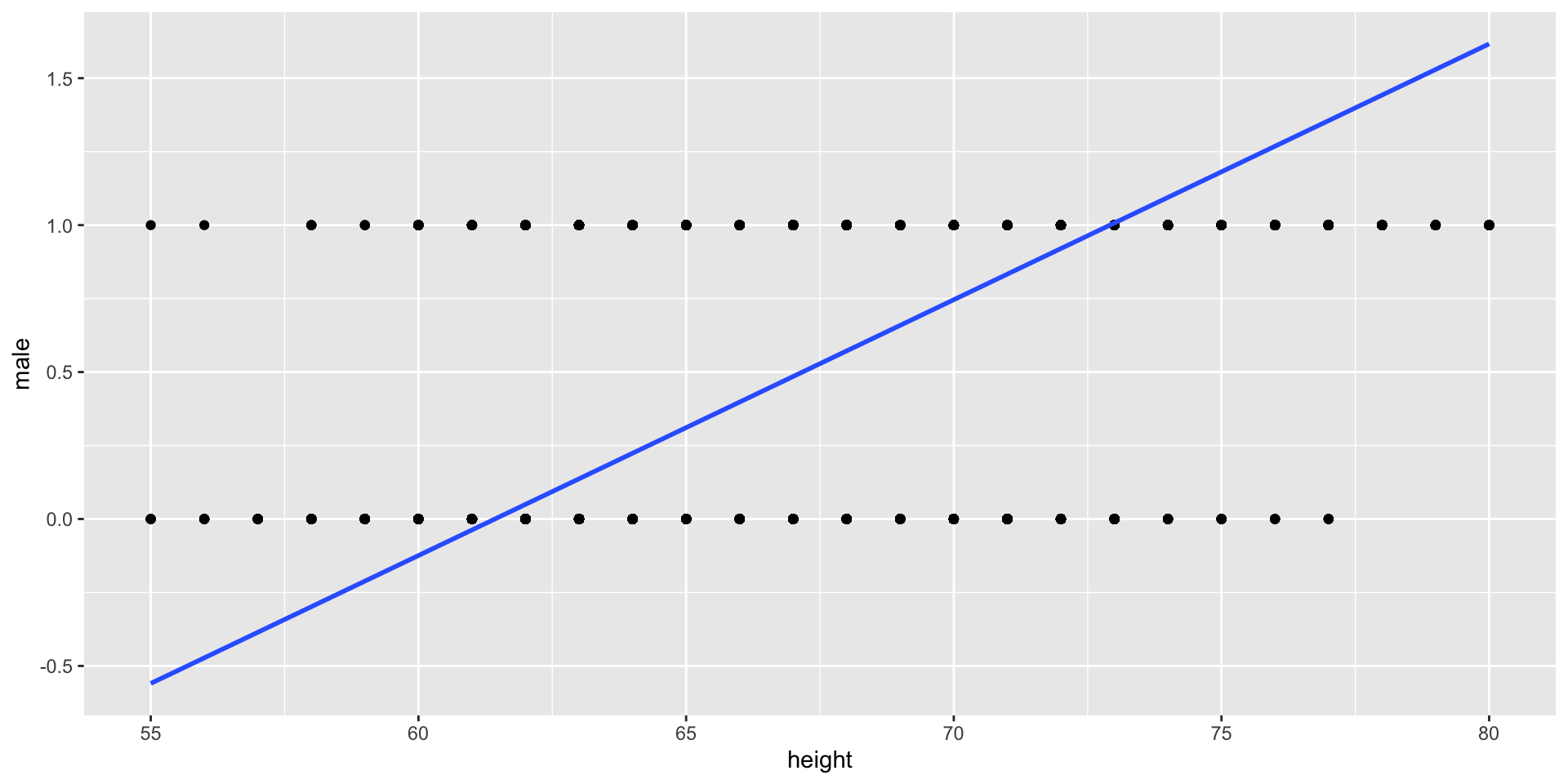
- A line is not a great fit to this data—it’s not even close to linear. And what does it mean to predict that
male= 0.7 (or 1.2)?
Logistic Regression
Instead of predicting whether someone is male, let’s predict the probability that they are male
In logistic regression, one level of \(Y\) is always called “success” and the other called “failure.” Since \(Y = 1\) for males, in our setup we have designated males as “success.” (You could also set \(Y = 1\) for females and call females “success.”)
Let’s fit a curve that is always between 0 and 1.
Odds and Probabilty
To fit the Logistic regression model we need to know the difference between odds and probability and how they relate.
When something has “even (1/1) odds,” the probability of success is 1/2.
When something has “2/1 odds,” the probability of success is 2/3.
When something has “3/2 odds,” the probability of success is 3/5.
In general, the odds of something happening are \(p/(1 − p)\).
Where \(p\) is the probability defined bewteen zero and one.
You can transform odds to probability: \[ \text{Odds} = \frac{3}{2} = \frac{3/(3+2)}{2/(3+2)} = \frac{3/5}{2/5} = \frac{p}{1-p} \]
If the odds are between zero and one they are not in your favor, \((1-p)>p\)
Let’s the explore this relation!
Probability vs odds vs log odds
| Probability \(p\) | Odds \(p/(1 − p)\) | Log odds \(\log(p/(1 − p))\) |
|---|---|---|
| 0 | 0 | \(-\infty\) |
| 0.25 | 0.33 | −1.10 |
| 0.5 | 1 | 0 |
| 0.75 | 3 | 1.10 |
| 0.8 | 4 | 1.39 |
| 0.9 | 9 | 2.20 |
| 0.95 | 19 | 2.94 |
| 1 | \(\infty\) | \(\infty\) |
- Probability is between zero and one.
- Odds are strictly positive (greater than zero).
- Log odds ranges the whole real line.
The logistic regression model
Logistic regression models the log odds of success \(p\) as a linear function of \(X\): \[ \log\left(\frac{p}{1-p}\right) = \beta_0 + \beta_1 \cdot X + e \]
This fits an “S-shaped” curve to the data
We’ll see what it looks like later
By making this choice, we have a series of benefits.
Let’s try it!
The logistic regression model
- We need a different function -
glm()(generalized linear models)
Call:
glm(formula = male ~ height, family = binomial, data = okcupid)

Coefficients:
              Estimate Std. Error z value Pr(>|z|)
(Intercept) -44.448609   0.357510  -124.3   <2e-16 ***
height        0.661904   0.005293   125.1   <2e-16 ***
---
Signif. codes:  0 '***' 0.001 '**' 0.01 '*' 0.05 '.' 0.1 ' ' 1

(Dispersion parameter for binomial family taken to be 1)

    Null deviance: 80654  on 59825  degrees of freedom
Residual deviance: 44637  on 59824  degrees of freedom
AIC: 44641

Number of Fisher Scoring iterations: 6- How ca we interpret this model?
The logistic regression model
The logistic regression output tells us that our prediction is \[ \log(\text{odds}) = \log\left(\frac{\widehat{p(\text{male})}}{1-\widehat{p(\text{male})}}\right) = −44.45 + 0.66 \cdot \text{height} \]
To get the probability we have to solve in terms \(\widehat{p(\text{male})}\)
The probability of being
malegivenheight: \[ \widehat{p(\text{male})} = \frac{\exp(−44.45 + 0.66 \cdot \text{height})}{1+ \exp(−44.45 + 0.66 \cdot \text{height})} \] where \(\exp()\) is the exponential function \(e^x\).
Let’s show this
Let \(\widehat{p} = \widehat{p(\text{male})}\), and \(\exp(X\widehat{\beta}) = \exp(−44.45 + 0.66 \cdot \text{height})\):
\[ \begin{eqnarray} \log\left(\frac{\widehat{p}}{1-\widehat{p}}\right) &=& X\widehat{\beta} \\ \exp\left(\log\left(\frac{\widehat{p}}{1-\widehat{p}}\right)\right) &=& \exp(X\widehat{\beta}) \\ \frac{\widehat{p}}{1-\widehat{p}} &=& \exp(X\widehat{\beta})\\ \widehat{p} &=& \exp(X\widehat{\beta})\cdot (1-\widehat{p})\\ \widehat{p} &=&\exp(X\widehat{\beta}) - \exp(X\widehat{\beta}) \cdot \widehat{p} \\ \widehat{p} &=& \frac{\exp(X\widehat{\beta})}{1 + \exp(X\widehat{\beta})} \end{eqnarray} \]
Visualizing the model
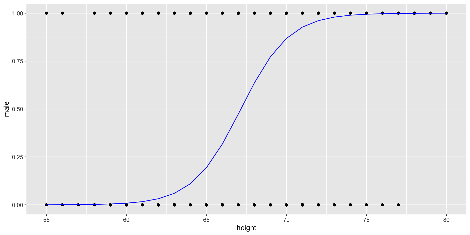
- How to interpret this curve?
- The blue line is \(\widehat{p(\text{male})}\), given the
height.
Interpreting the coefficients
Our prediction equation is:
\[ \log(\text{odds}) = \log\left(\frac{\widehat{p(\text{male})}}{1-\widehat{p(\text{male})}}\right) = −44.45 + 0.66 \cdot \text{height} \]
Let’s start with some basic, but not particularly useful, interpretations:
When
height= 0, we predict that the log odds will be -44.45 , so the probability of male is predicted to be very close to 0%.When
heightincreases by 1 inch, we predict that the log odds of being male will increase by 0.66.Instead of log odds is better to have the interpretation in odds.
Interpreting the coefficients
Let’s rewrite the prediction equation as:
Predicted odds of male, \(\exp(−44.45 + 0.66 \cdot \text{height})\).
Increasing height by 1 inch will multiply the odds by \(\exp(0.66) = 1.94\); i.e., increase the odds by 94%.
In summary, \[(\exp(\widehat{\beta}) - 1)\times 100 = \text{percentage change in odds}.\]
Increasing height by 2 inches will multiply the odds by \(\exp(2\cdot0.66) = 3.76\); i.e., increase the odds by 276%.
Odds equal to 1 indicate an one-to-one chance.
Making predictions
- What is the probability of being male given we have a height of 69.
- Using the probability equation in R:
\[ \widehat{p(\text{male})} = \frac{\exp(−44.45 + 0.66 \cdot 69)}{1+ \exp(−44.45 + 0.66 \cdot 69)} = 0.77 \]
Adding more predictors
Adding another predictor: can we do better?
Just like with a linear regression model, we can add additional predictors to the model.
Our interpretation of the coefficients in multiple logistic regression is similar to multiple linear regression, in the sense that each coefficient represents the predicted effect of one \(X\) on \(Y\), holding the other \(X\) variables constant.
How good is our model?
- Unfortunately, the typical root mean squared error, RSE metric isn’t available for logistic regression.
- However, there are many metrics that indicate model fit.
- But: most of these metrics are difficult to interpret, so we’ll focus on something simpler to interpret and communicate.
Accuracy of the model
We could use our model to make a prediction of sex based on the probability.
Suppose we say that our prediction is: \[ \text{Prediction} = \begin{cases} \text{male}, & \text{if $\widehat{P(\text{male})} \geq 0.5$}, \\ \text{female}, & \text{if $\widehat{P(\text{male})} < 0.5$}. \\ \end{cases} \]
Given a threshold of 0.5, now we can compute the fraction of individuals whose sex we correctly predicted.
For males and females.
This is known as the accuracy of the model.
Accuracy of the model
We can use the
xtabsfunction to get the accuracy:We add we the number of correctly predicted groups for both male and female, and divide by the total of observations.
okcupid = okcupid %>%
  mutate(predict.sex = ifelse(predict(model, type="response") >= 0.5,"m","f"))
xtabs(~ predict.sex + sex,okcupid) %>%
  addmargins()
sex
predict.sex f m Sum
f 19466 5494 24960
m 4623 30243 34866
Sum 24089 35737 59826- Correctly predicted that is female - 19466
- Correctly predicted that is male - 30243
- Total number of individuals in the sample - 59826
- The accuracy is (19466 + 30243)/59826 = 0.831, or 83%
Confusion Matrix
- The table from
xtabsis also called a Confusion matrix
| Actual failure | Actual success | |
|---|---|---|
| Model predicts failure | True negative | False negative |
| Model predicts success | False positive | True positive |
- True positives: predicting male for someone that is male
- True negatives: predicting female for someone that is female
- False positives: predicting male for someone that is female
- False negatives: predicting female for someone that is male
- If we had designated female as 1 and male as 0, these would have switched
- So Accuracy = (True negative + True positive)/(Total cases)
Accuracy of the model
Suppose that the Amazon is trying to build a model to predict which costumers buy a certain product:
Suppose that 0.01% of people are costumers of this product (the product is really expensive / high revenue)
A “null” or “no-brainer” model that predicts that no one is a costumer will be 99.99% accurate.
The revenue coming from our model would be zero.
But the model could make two different kinds of prediction errors:
False positive: predicting someone is a customer when they really are not
False negative: predicting someone is not a customer when they really are
These two measures give us a better idea of the predictive power of our model.
False positive rate
The false positive rate is the proportion of actual failures where the model predicted success.
           sex
predict.sex     f     m   Sum
        f   19466  5494 24960
        m    4623 30243 34866
Sum 24089 35737 59826- False Positives - predicting someone is a male when they really are female
- Actual failure - number of cases that are female
- False positive rate = False positives/ Actual failure
- In our model, the false positive rate is 4623/24089 = 0.19
False negative rate
The false negative rate is the proportion of actual successes where the model predicted failure.
           sex
predict.sex     f     m   Sum
        f   19466  5494 24960
        m    4623 30243 34866
Sum 24089 35737 59826- False Negatives - predicting someone is a female when they really are male
- Actual success - number of cases that are male
- False negative rate = False negatives/ Actual success
- In our model, the false positive rate is 5494/35737 = 0.15
Changing rates
How do we reduce false positive/negative rates?
- Instead of using 50% as a cutoff probability to decide when to predict success, use a higher (or lower) probability.
- For example, we could have the model predict that someone is male only if \(\widehat{p(\text{male})} \geq 0.8\), instead of 0.5:
okcupid = okcupid %>%
  mutate(predict.sex = ifelse(predict(model, type="response") >= 0.8,"m","f"))
xtabs(~ predict.sex + sex,okcupid) %>%
  addmargins()
sex
predict.sex f m Sum
f 22650 12938 35588
m 1439 22799 24238
Sum 24089 35737 59826- Accuracy = (21425+26753)/59826 = 0.76
- False positive rate = 2664/24089 = 0.06
- False negative rate = 8984/59826 = 0.36
Prediction Trade off
We can decrease the false positive rate, but at the expense of increasing the false negative rate.
Or we can decrease the false negative rate, but at the expense of increasing the false positive rate.
We might choose a cutoff probability other than 50% based on our assessment of the relative costs of the two different kinds of errors.
Summary
In a logistic regression model, the response variable is binary, taking values of either zero or one.
The model estimates the log odds of the event associated with a response of one.
The model’s effects are interpreted in terms of odds.
Predictions are expressed as probabilities.
The performance of the model is evaluated based on its prediction accuracy.
![]()