Data Science for Business Applications
Causal Inference
- Natural Experiments (RCTs in the wild).
- Always check for balance! (All things equal!)
- Difference-in-Differences (Diff-in-Diff):
- How we can use two wrong estimates to get a right one.
- Assumptions behind DD (Parallel changes).
Regression Discontinuity Design
- What will we learn today?
- Regression Discontinuity Design (RDD)
- How can we use discontinuities to recover causal effects?
- Assumptions behind RDD designs.
Introduction
Arbitrary rules determine treatment assignment:
If you are above a threshold, you are assigned to treatment, and if your below, you are not (or vice versa)
Geographic discontinuities
Time discontinuities
Voting discontinuities
You can find discontinuities everywhere!
Example: Cohort size
- Many people argue that smaller classes lead to better learning outcomes compared to large classes.
- But why can’t we just compare test scores of students in small classes and students in large classes?
- Angrist & Levy (1999) studied this by taking advantage of a rule in Israeli schools, where cohorts of >40 students are split into two smaller classes
Example: Cohort size
Key idea: Students in cohorts just below 40 students are essentially identical to students in cohorts just above 40, but the ones in the latter group will get a smaller class.
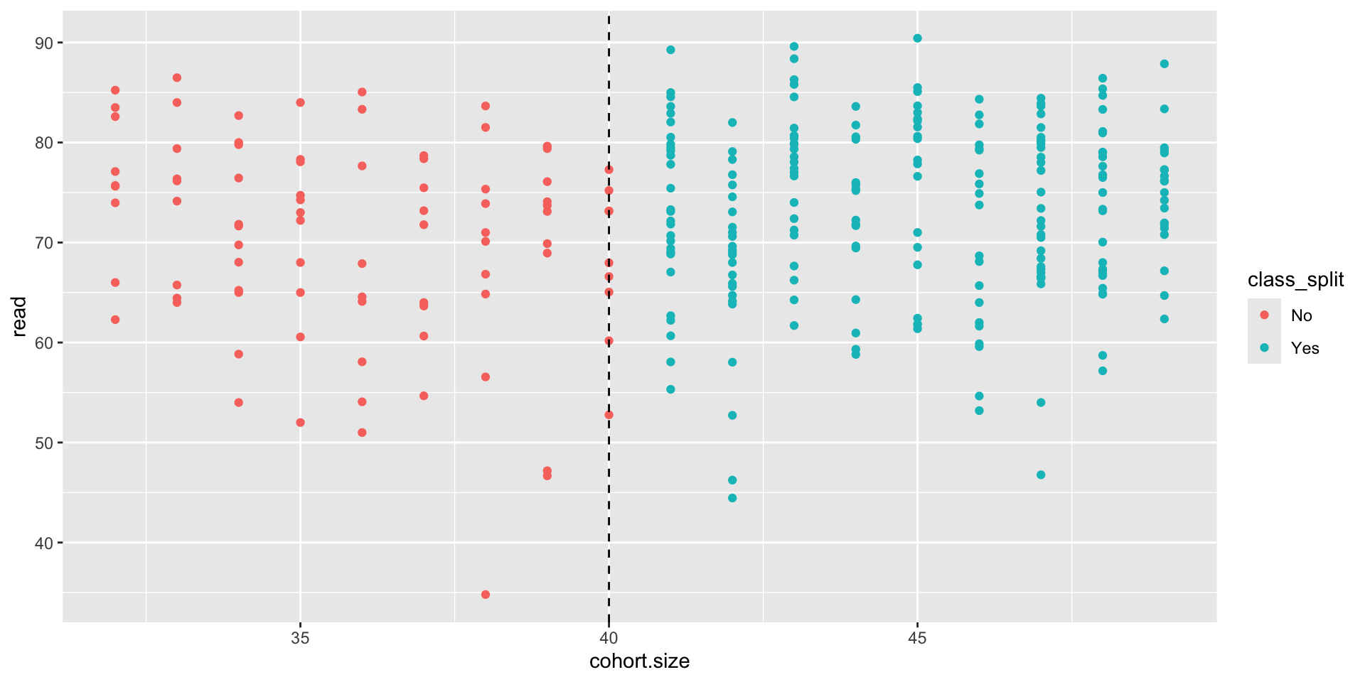
- Is there a difference in the reading score between larger and smaller classes?
Creating the RDD model
Define a treatment variable: \[\begin{equation} T = \begin{cases} 1, \quad \text{split cohort},\\ 0, \quad \text{intact cohort} \end{cases} \end{equation}\]
Recenter the selection variable so the cutoff is at 0: \[\begin{equation} X = (\texttt{cohort.size}) − 40 \end{equation}\]
Then fit a model predicting reading scores from both \(X\) and \(T\): \[\begin{equation} \widehat{Y} = \widehat{\beta}_{0} + \widehat{\beta}_1 X + \widehat{\beta}_2 T \end{equation}\]
- The coefficient \(\widehat{\beta}_2\) of \(T\) is the causal effect we’re looking for!
RDD model
class_1999 = class_1999 %>%
  mutate(treatment=ifelse(cohort.size > 40, 1, 0),
         selection=(cohort.size - 40))

rdd1 <- lm(read ~ selection + treatment, data=class_1999)
summary(rdd1)
Call:
lm(formula = read ~ selection + treatment, data = class_1999)

Residuals:
    Min      1Q  Median      3Q     Max
-35.195  -5.572   1.537   6.617  17.269

Coefficients:
            Estimate Std. Error t value Pr(>|t|)
(Intercept)  69.7556     1.2697  54.939   <2e-16 ***
selection    -0.1195     0.2020  -0.592   0.5545
treatment     4.0031     2.1511   1.861   0.0638 .
---
Signif. codes:  0 '***' 0.001 '**' 0.01 '*' 0.05 '.' 0.1 ' ' 1

Residual standard error: 9.135 on 294 degrees of freedom
Multiple R-squared:  0.02237,   Adjusted R-squared:  0.01572
F-statistic: 3.363 on 2 and 294 DF, p-value: 0.03596- The effect of the treatment is an increase of \(\widehat{\beta}_2 = 4\) points in the reading score if the students.
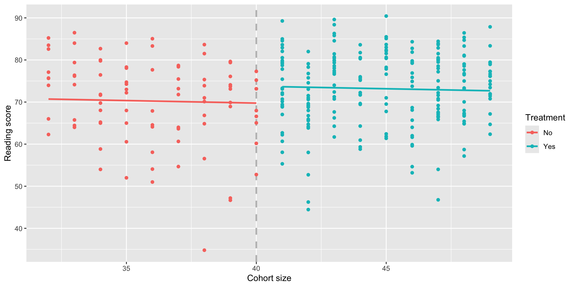
Pre vs post comparison
Our first RDD model is forcing the two lines to have the same slope; that isn’t a great fit for the data:
RDD and interactions
To allow the two slopes to be different, we can add an interaction term to allow the slope of \(X\) to be different for \(T = 0\) (cohort kept intact) and \(T = 1\) (cohort split into smaller classes): \[\begin{equation} \widehat{Y} = \widehat{\beta}_0 + \widehat{\beta}_1 X + \widehat{\beta}_2 T + \widehat{\beta}_3 T\cdot X \end{equation}\]
Again, the slope of \(\widehat{\beta}_2\) is our estimate of the causal effect of the treatment.
RDD with interactions
Call:
lm(formula = read ~ selection * treatment, data = class_1999)

Residuals:
    Min      1Q  Median      3Q     Max
-33.618  -6.102   1.341   6.922  17.249

Coefficients:
                    Estimate Std. Error t value Pr(>|t|)
(Intercept)          66.6294     1.8141  36.729   <2e-16 ***
selection            -0.8945     0.3806  -2.350   0.0194 *
treatment             5.6641     2.2439   2.524   0.0121 *
selection:treatment   1.0720     0.4477   2.395   0.0173 *
---
Signif. codes:  0 '***' 0.001 '**' 0.01 '*' 0.05 '.' 0.1 ' ' 1

Residual standard error: 9.063 on 293 degrees of freedom
Multiple R-squared:  0.04113,   Adjusted R-squared:  0.03132
F-statistic: 4.19 on 3 and 293 DF, p-value: 0.00634- From our data we an conclude that smaller class sizes cause reading scores to increase by about 5.7 points.
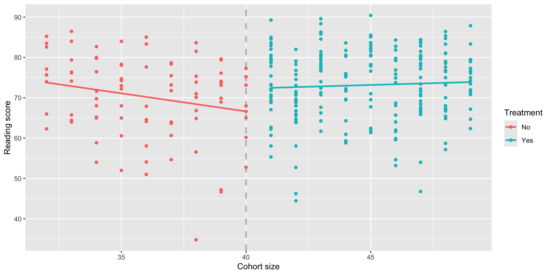
RDD with interactions
More flexibility with the interaction gives the model a better fit in relation to the data:
Conclusion
- RDD is usually great for internal validity, but there are lots of threats to external validity.
- Why this statement holds?
- For example, would this generalize to different grade levels? Schools outside of Israel?
Example: Sales
- You are managing a retail store and notice that sales are low in the mornings, so you want to improve those numbers.
- A store gives a 10% discount to the first 1,000 customers that arrive.
- Is this a good candidate for regression discontinuity?
- Let’s look at the data.
Example: Sales
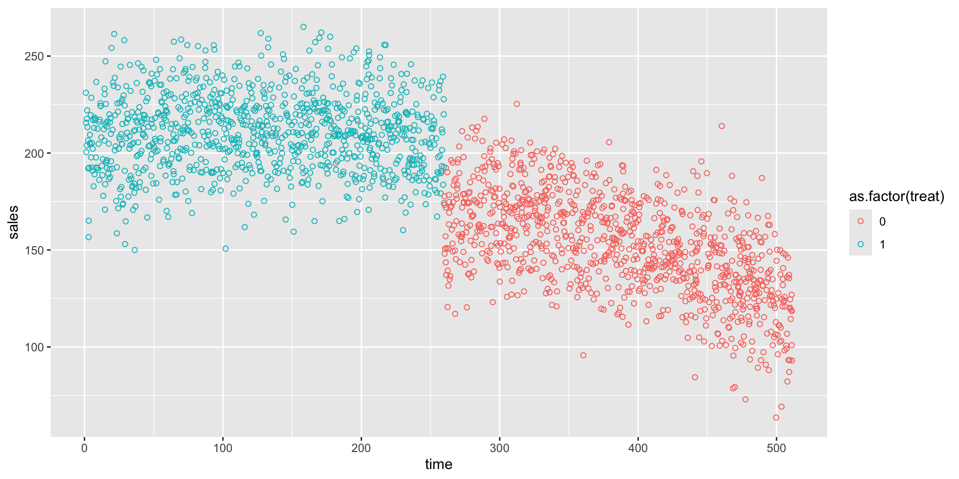
- Sales in relation to time since the opening of the store in minutes.
- The store receives its 1,000th customer around 260 minutes after opening (around 4.3 hours).
Creating the RDD model
Define a treatment variable: \[\begin{equation} T = \begin{cases} 1, \quad \text{promotion}\\ 0, \quad \text{no promotion} \end{cases} \end{equation}\]
Recenter the selection variable so the cutoff is at 0: \[\begin{equation} X = (\texttt{time}) - 260 \end{equation}\]
Then fit a model predicting the sales of a customer from both \(X\) and \(T\): \[\begin{equation} \widehat{Y} = \widehat{\beta}_{0} + \widehat{\beta}_1 X + \widehat{\beta}_2 T \end{equation}\]
- The coefficient \(\widehat{\beta}_2\) is the causal effect we are looking for!
RDD model
sales = sales %>%
  mutate(selection=(time - 260))

rdd_sales <- lm(sales ~ selection + treat, data=sales)
summary(rdd_sales)
Call:
lm(formula = sales ~ selection + treat, data = sales)

Residuals:
   Min     1Q Median     3Q    Max
-77.32 -14.62   0.14  14.56  68.95

Coefficients:
             Estimate Std. Error t value Pr(>|t|)
(Intercept) 165.61482    1.08422  152.75   <2e-16 ***
selection    -0.10294    0.00661  -15.57   <2e-16 ***
treat        31.52628    1.95845   16.10   <2e-16 ***
---
Signif. codes:  0 '***' 0.001 '**' 0.01 '*' 0.05 '.' 0.1 ' ' 1

Residual standard error: 21.82 on 1997 degrees of freedom
Multiple R-squared:  0.6539,    Adjusted R-squared:  0.6535
F-statistic: 1886 on 2 and 1997 DF, p-value: < 2.2e-16- On average, providing a 10% discount increases sales by $31.30 for the 1,000 customers, compared to not having a discount.
RDD model
A more flexible RDD model
As in the first example, we have that two lines of the RDD model have the same slope.
We can make this model more flexible by adding an interaction term.
To allow the two slopes to be different, we can add an interaction term to allow the slope of \(X\) to be different for \(T = 0\) (after 1,000th customer) and \(T = 1\) (first thousand customers):
\[\begin{equation} \widehat{Y} = \widehat{\beta}_0 + \widehat{\beta}_1 \, X + \widehat{\beta}_2 \, T + \widehat{\beta}_3 \, X\cdot T \end{equation}\]
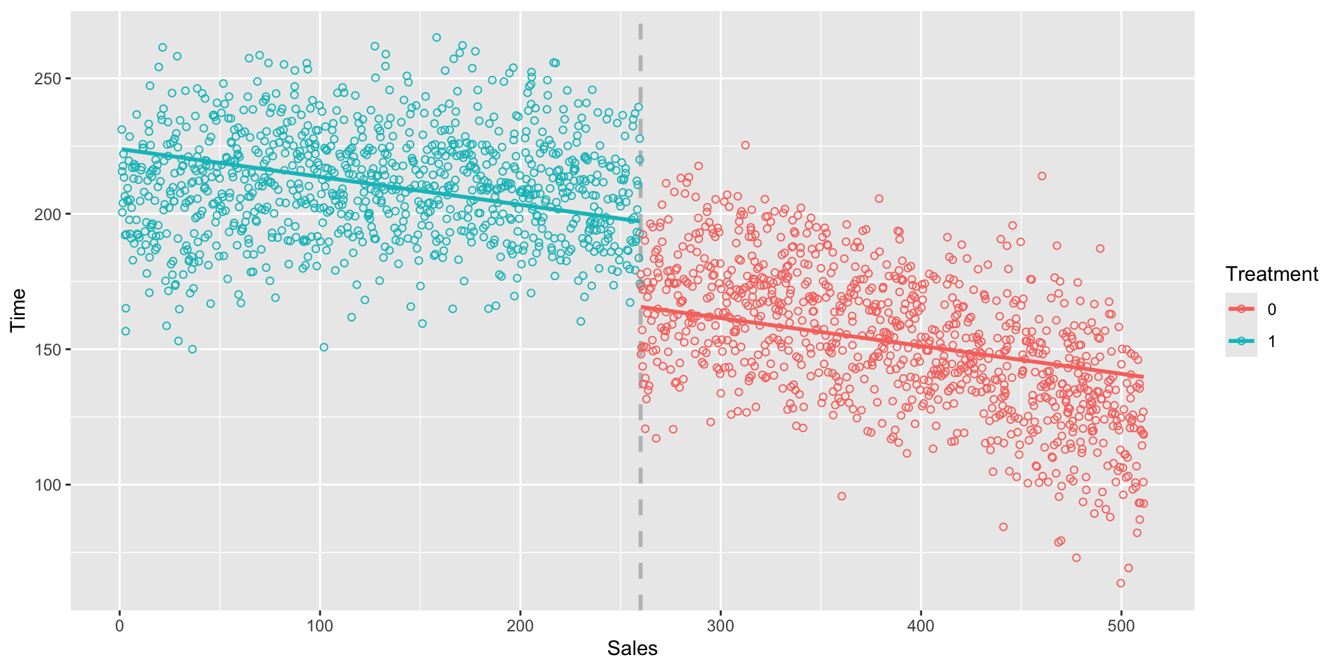
RDD with interaction
Call:
lm(formula = sales ~ selection * treat, data = sales)

Residuals:
    Min      1Q  Median      3Q     Max
-65.738 -13.940   0.051  13.538  76.515

Coefficients:
                  Estimate Std. Error t value Pr(>|t|)
(Intercept)     178.574245   1.297815  137.60   <2e-16 ***
selection        -0.205355   0.008882  -23.12   <2e-16 ***
treat            31.399196   1.842316   17.04   <2e-16 ***
selection:treat   0.200845   0.012438   16.15   <2e-16 ***
---
Signif. codes:  0 '***' 0.001 '**' 0.01 '*' 0.05 '.' 0.1 ' ' 1

Residual standard error: 20.52 on 1996 degrees of freedom
Multiple R-squared:  0.6939,    Adjusted R-squared:  0.6934
F-statistic: 1508 on 3 and 1996 DF, p-value: < 2.2e-16- On average, providing a 10% discount increases sales by $33.10 for the 1,000 customers, compared to not having a discount.
RDD with interaction
- We have different slopes, for before and after the treatment.

Conclusion
- Again, RDD is usually great for internal validity, but there are lots of threats to external validity.
- For example, would this generalize to different types of products? Same store, but a different location?
![]()