[1] 0.189Data Science for Business Applications
Class 01 - Course Syllabus and Simple Regression
Course Overview
Course Overview
- Data and analytics are fundamental sources of value creation for organizations and their stakeholders
- We’ll practice applying sophisticated statistical methods to address complex business questions under conditions of uncertainty
- You’ll learn to analyze data and communicate results in plain language so your organization can gain insight and take better action
- You’ll build hands-on skills in RStudio, a leading platform for data analysis and visualization used across industries
Course Overview
- This course carries the Quantitative Reasoning (QR) Flag
- QR courses equip you with skills for understanding quantitative methods and frameworks you’ll encounter regularly in your adult and professional life
Course Logistics
University Course Catalog Description
- Data science for business applications at the intermediate level:
- Building and validating predictive models
- Advanced regression modeling
- Models for binary outcomes
- Causal inference
- The equivalent of two lecture hours a week for one semester
- Offered on the letter-grade basis only; restricted to McCombs students
Course Materials
- No textbook required for this course
- You will need a laptop with a modern, updated operating system (macOS or Windows)
- Bring it to every class meeting
- We will use RStudio during most (if not all) class sessions
- If you don’t have R/RStudio installed already from STA 301, you can download them for free

Assignments and Grading
Assignments and Grading
- Your course grade is the sum of points earned across all components below
- We will not curve individual assignments
- Because STA 235 is a core course, letter-grade cutoffs will target an overall course GPA of approximately 3.0-3.2
- Cutoffs will be finalized at the end of the semester but will be set no higher than the scale on the next slide
Grading Scale
| Cutoff (/1000) | Grade |
|---|---|
| 930 | A |
| 900 | A- |
| 870 | B+ |
| 830 | B |
| 800 | B- |
| 770 | C+ |
| Cutoff (/1000) | Grade |
|---|---|
| 730 | C |
| 700 | C- |
| 670 | D+ |
| 630 | D |
| 600 | D- |
Pre-class Preparation (45 points)
- Come to class prepared so class time isn’t the first time you see the material
- We use Perusall to discuss short readings/videos with classmates before each class
- While reading/watching, you can:
- Highlight confusing text and ask a question
- Answer a classmate’s question
- Share insights, outside knowledge, thoughts, or opinions
- Full credit as long as you make a reasonable effort to meaningfully engage
Class Participation (40 points)
- Practice is essential, and the best time to start is during class
- We use Canvas for in-class “clicker” questions and other collaborative activities
- Scored on participation only, not correctness
- Respond to at least 75% of the questions over the semester for full credit
Post-class Practice (5 points each, 55 points total)
- Weekly homework on material covered in class that week
- Submitted on Canvas, due at 11:59 PM the day before each class
- Credit is for completion only, with unlimited attempts and feedback
- Form study groups and discuss with classmates — but simply copying answers won’t help you learn
Checkpoint Quizzes (40 points each, 440 points total)
- Most classes start with a 15-minute Checkpoint Quiz on the previous week’s material
- You may use one 8.5” x 11” reference page (both sides OK) during quizzes
Team Labs (40 points each, 120 points total)
- 3 class sessions are devoted to Team Labs
- Work with your team through a set of questions to practice material learned so far
- Team Labs also serve as practice for the Team Cases
Team Cases (100 points each, 300 points total)
- An opportunity to demonstrate your skills on an authentic business analytics task
- Your team signs up for a time slot outside of class for each of the 3 Team Cases
- You’ll be given a data set and business case, analyze it with your group, and produce slide(s) answering the business questions
- Team members are randomly selected to present and answer questions
Virtual Tokens
- Each student starts the semester with 3 virtual tokens
- Spend a token to discard a missed assignment score and receive a makeup assignment (often an oral assessment)
- Once used, your original score is replaced by the makeup score — higher or lower
- Excused absences verified by Student Emergency Services don’t require a token
- No late work is accepted outside of these parameters
Teamwork
Teamwork
- Team-based activities (Team Labs and Team Cases) are integrated throughout the course
- You’ll be assigned to a team after the first few weeks; your team stays the same for the semester
- Team members generally receive the same score for team-based work
- Individual scores may be adjusted up or down if circumstances warrant
- Missing a Team Lab/Case without a token results in a zero
Teamwork
- If your team wants to replace an unsatisfactory score with a token, every team member must spend one of their tokens
- Check in with your teammates throughout the semester:
- Am I satisfied with my teammates’ work? Are they satisfied with mine?
- Open, honest dialogue now pays off later when working with teams in your career
- What personal characteristics about an instructor do you think are predictive of the scores they receive on student evaluations?
Hamermesh & Parker (2005) Data Set
- Student evaluations of \(N=463\) instructors at UT Austin, 2000-2002
- For each instructor:
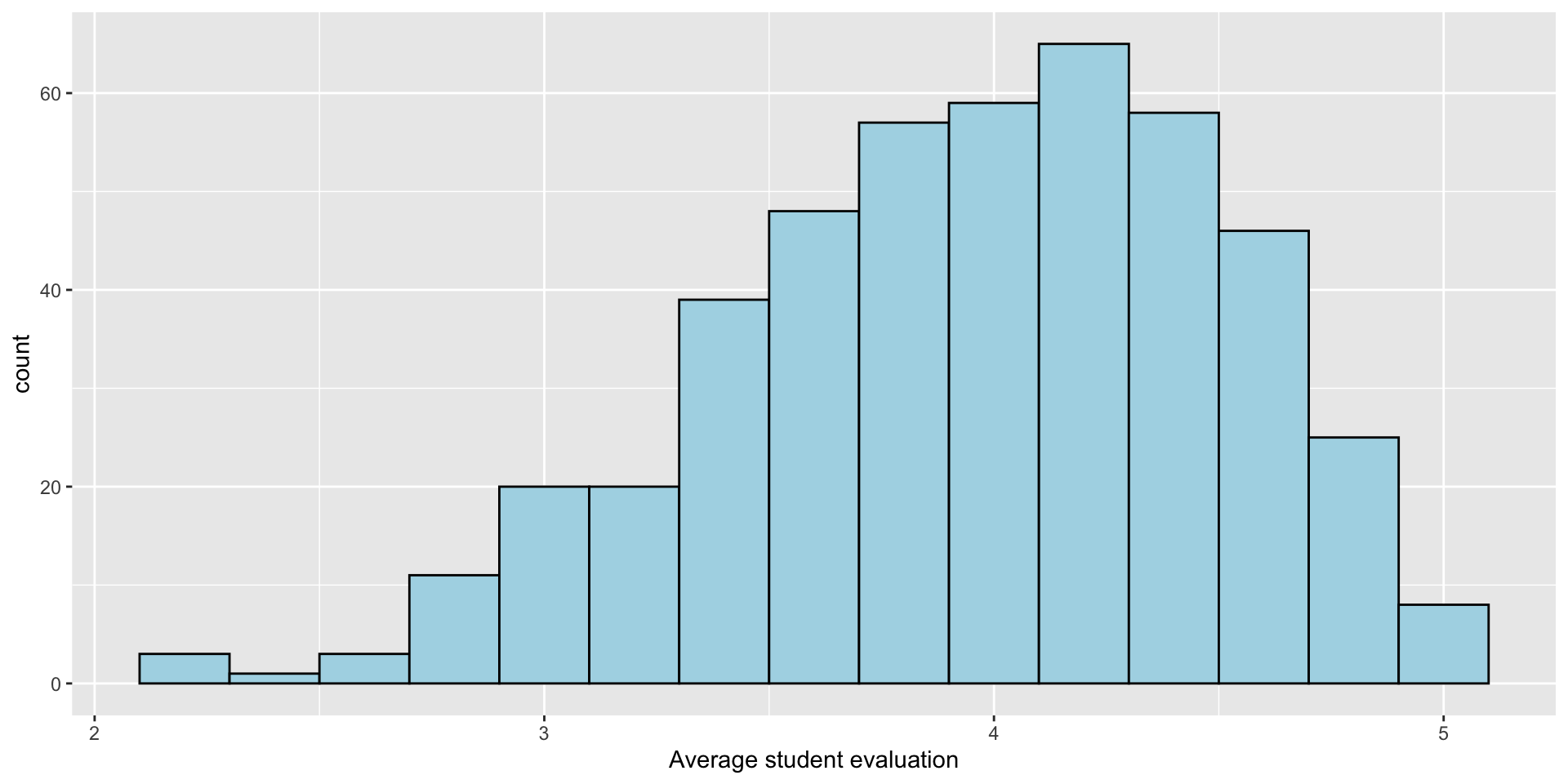
- \(\texttt{eval}\): average student evaluation of teacher
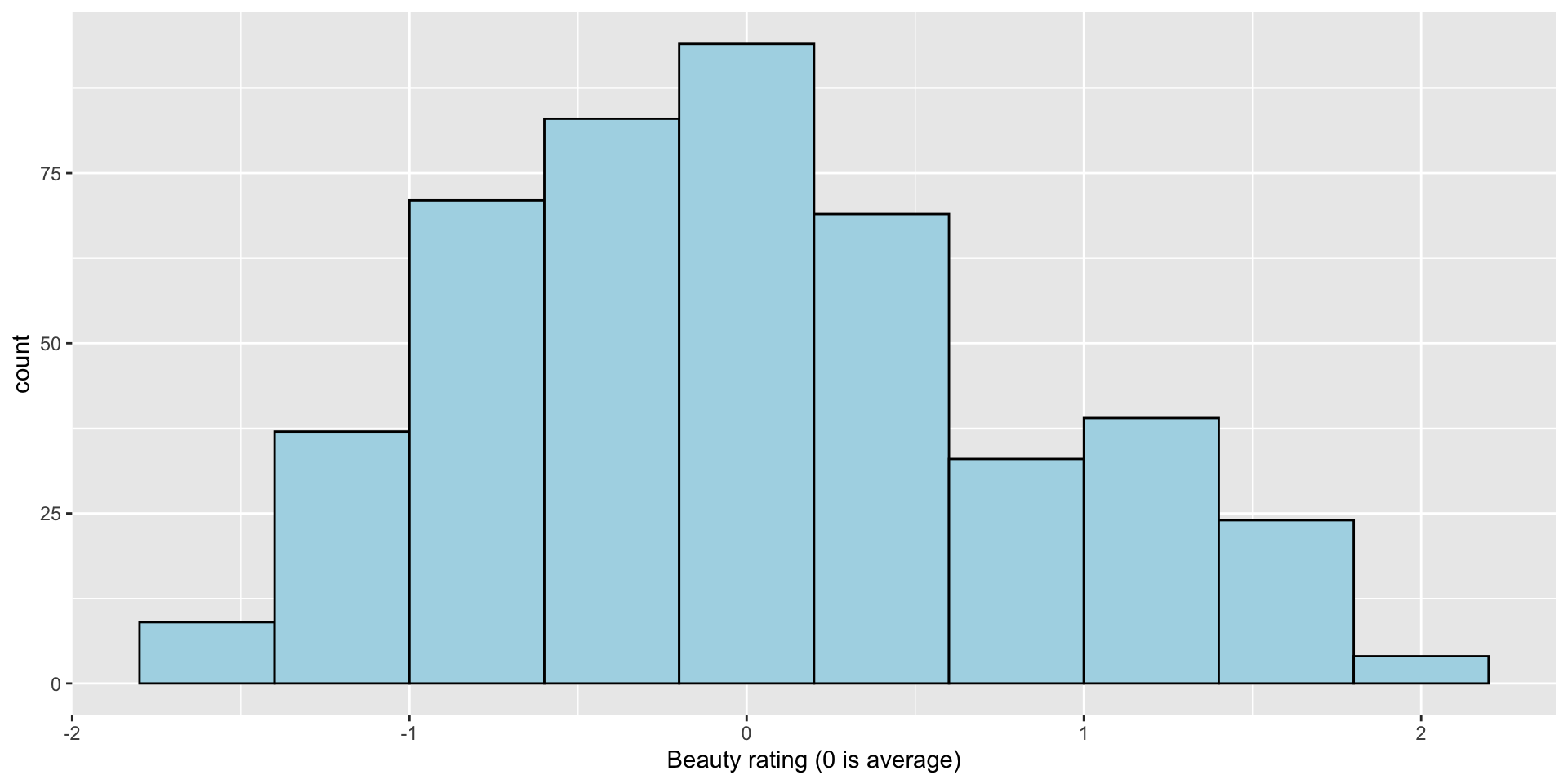
- \(\texttt{beauty}\): average beauty score from a six-student panel
- \(\texttt{gender}\): male or female
- \(\texttt{credits}\): single- or multi-credit course
- \(\texttt{age}\): age of instructor
- (and more…)
Explore the data: \(\texttt{eval}\)
Explore the data: \(\texttt{beauty}\)
- Do you think there is a positive or negative relationship between beauty and teaching ratings?
Explore the data
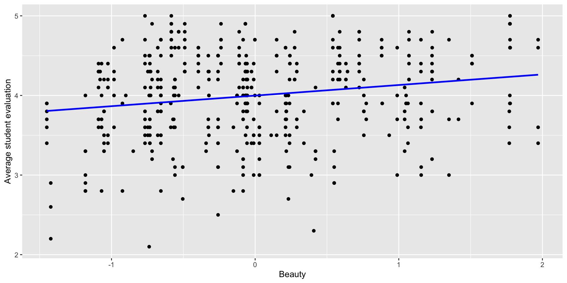
The correlation \(r\) between two variables \(X\) and \(Y\) measures the strength of the linear relationship between them. Correlation ranges from \(-1\) (perfect negative relationship) to \(0\) (no relationship) to \(1\) (perfect positive relationship).
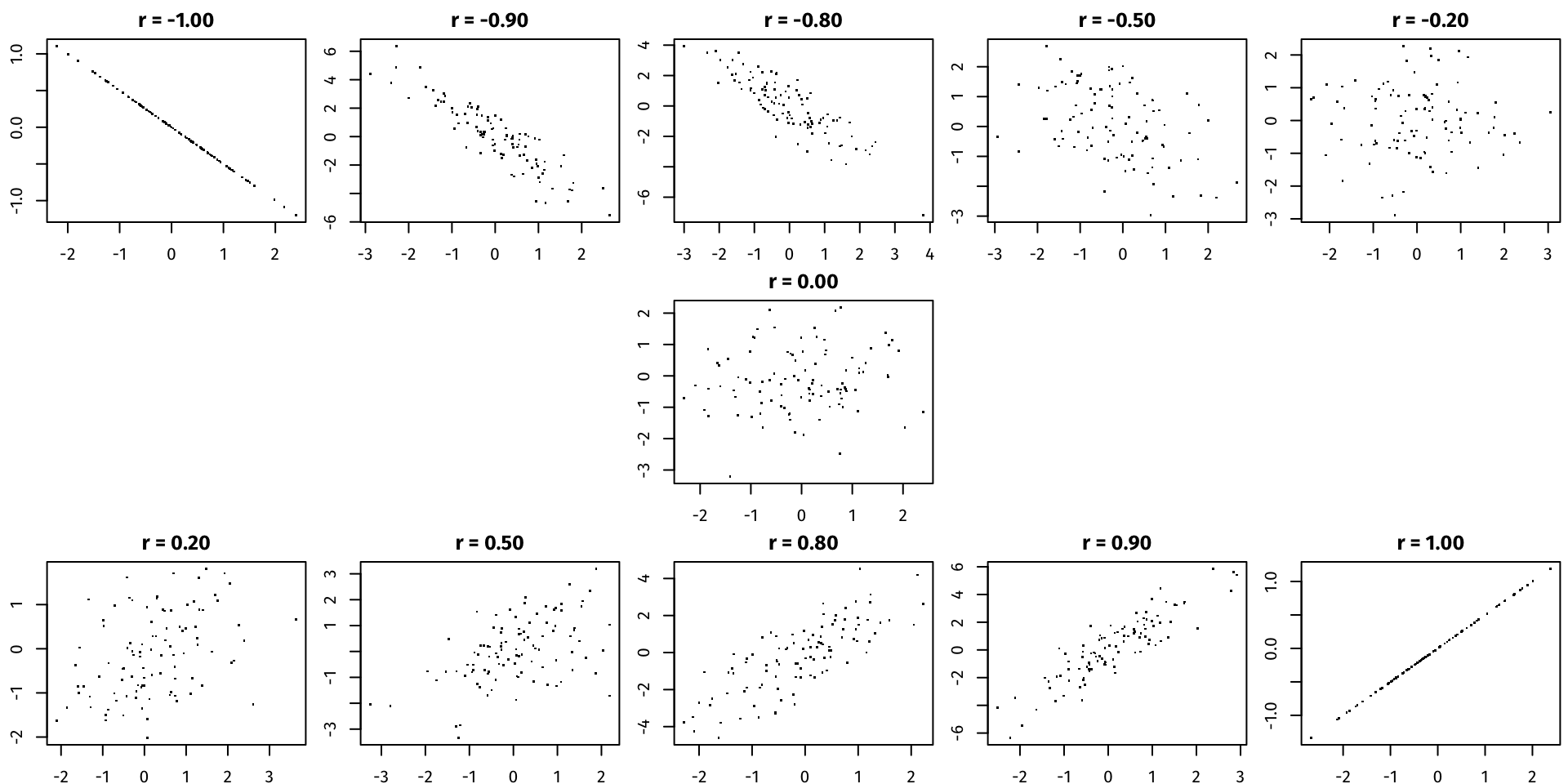
Correlation
- How can we interpret this?
- The
$sign accesses the variables in the data setprofs.csv.
The simple regression fit
Call:
lm(formula = eval ~ beauty, data = profs)

Residuals:
    Min      1Q  Median      3Q     Max
-1.8002 -0.3630  0.0725  0.4021  1.1037

Coefficients:
            Estimate Std. Error t value             Pr(>|t|)
(Intercept)   3.9983     0.0253  157.73 < 0.0000000000000002 ***
beauty        0.1330     0.0322    4.13             0.000042 ***
---
Signif. codes:  0 '***' 0.001 '**' 0.01 '*' 0.05 '.' 0.1 ' ' 1

Residual standard error: 0.545 on 461 degrees of freedom
Multiple R-squared:  0.0357,    Adjusted R-squared:  0.0336
F-statistic: 17.1 on 1 and 461 DF, p-value: 0.0000425(Intercept) beauty
3.998 0.133 Interpreting the coefficients
- Intercept:
- When beauty = 0 (average), predicted eval = 3.998 points
- The average evaluation for an average-looking instructor
- Meaningful this time!
- Slope:
- For a one unit (standard deviation) increase in beauty, the predicted eval increases by 0.13 points
- Comparing two instructors who differ by 1 SD on beauty, on average the more attractive instructor has an eval score 0.13 points higher
Is this the whole story?
Probably not!
- Lots of other predictors to consider
- Could the positive association be due to another variable that isn’t in the model yet (think bedrooms and living area)?
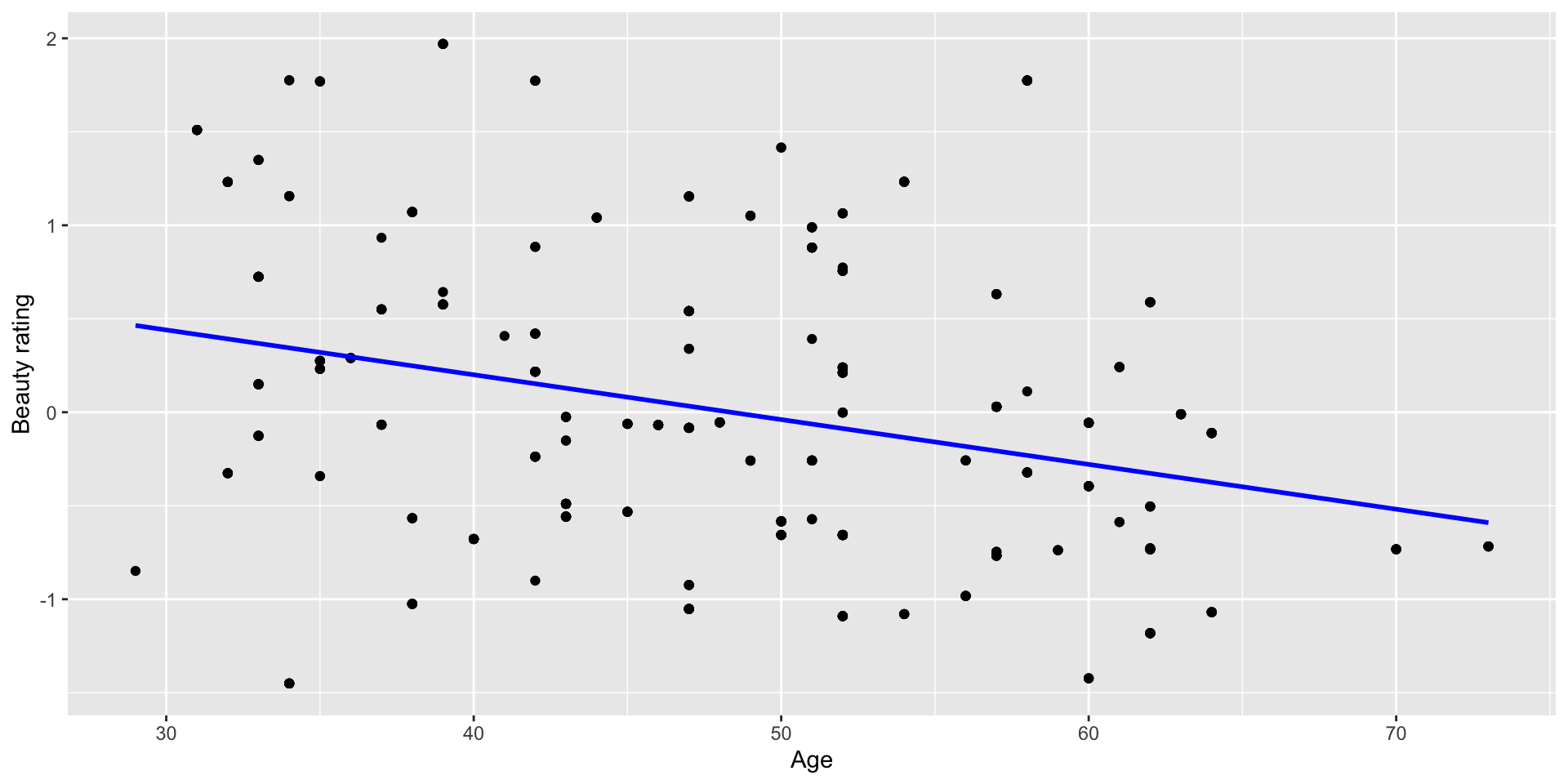
- Age might be important here – how? - On average, older instructors are less hot - As they age instructors might get better at teaching (experience) – or worse (stale or out of touch)
Is age actually correlated with beauty?
Multiple regression: eval on beauty and age
Call:
lm(formula = eval ~ beauty + age, data = profs)

Residuals:
    Min      1Q  Median      3Q     Max
-1.8024 -0.3651  0.0741  0.3991  1.1021

Coefficients:
            Estimate Std. Error t value             Pr(>|t|)
(Intercept) 3.984401   0.133730   29.79 < 0.0000000000000002 ***
beauty      0.134063   0.033744    3.97             0.000082 ***
age         0.000287   0.002715    0.11                 0.92
---
Signif. codes:  0 '***' 0.001 '**' 0.01 '*' 0.05 '.' 0.1 ' ' 1

Residual standard error: 0.546 on 460 degrees of freedom
Multiple R-squared:  0.0358,    Adjusted R-squared:  0.0316
F-statistic: 8.53 on 2 and 460 DF,  p-value: 0.00023
Interpreting the coefficients
- In this case, whether we compare instructors of the same age or not, we get the same answer: Hotter instructors get higher evaluations on average.
- Good(ish) news – we ruled out one alternative explanation for the association between beauty and eval
- Are there others?
Summary
- As we add or remove variables in regression models, the coefficients on other variables can go up, down, or stay about the same
- It all depends on the relationships among the predictors and between the predictors and the outcome
- To understand what’s happening – and which variables we should include to estimate the right effect – we need to understand the effect we’re estimating and whether it’s the one we want
- In a few weeks we’ll learn how to build models that estimate the right effects, and how to build the best predictve models (these aren’t always the same!)
Next time: Errors and uncertainty
The other missing part of the story:
- Does the association between beauty and evals hold among ALL instructors, or just in this sample? - Could we be looking at a chance association that would disappear if we could get data on everyone?
- How accurately can we predict the sale price of a house from its size and other factors? - How do we quantify prediction errors? Even with many variables our predictions will be off by some amount. How wrong should we expect to be?
