Error, Uncertainty and the Linear Model

STA 235 Lecture 2

Henrique Bolfarine

University of Texas at Austin

2026-01-22

Posit Cloud vs RStudio

Originally we had planned for you to use Posit Cloud not just for quizzes/exams, but for in-class work and homework too
It turns out that the limits on the free version of Posit Cloud are too restrictive
New plan:
- You can use Posit Cloud for quizzes/exams
- You can use RStudio (install on your computer) for in-class work and homework

Measuring prediction error

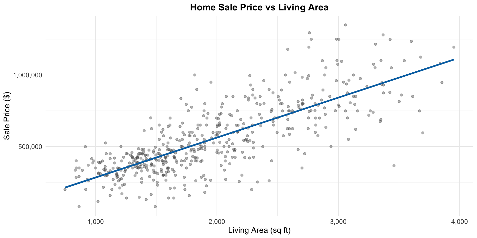
Predicting price from area

Residuals and fitted values

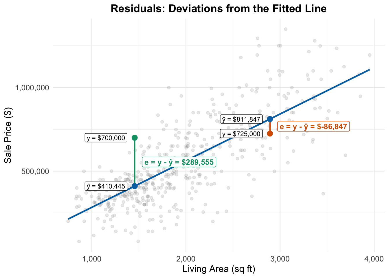
The fitted value (“y hat”) for observation i is the predicted value from the regression line: \widehat{y}_i = \widehat{\beta_0} + \widehat{\beta_1} \times \text{area}_i
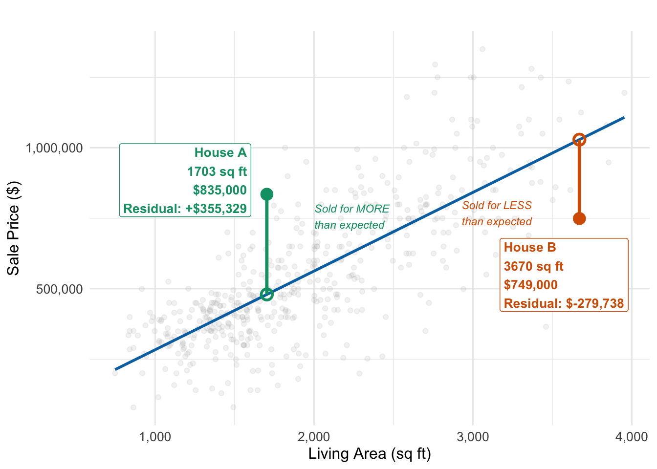
The residual is the corresponding prediction error: e_i = y_i - \widehat{y}_i = \text{observed price} - \text{predicted price}
The fitted line tells us about the part of price predictable from area
The residuals tell us about the part of price not predictable from area

Visualizing residuals and fitted values

What does a residual tell us?

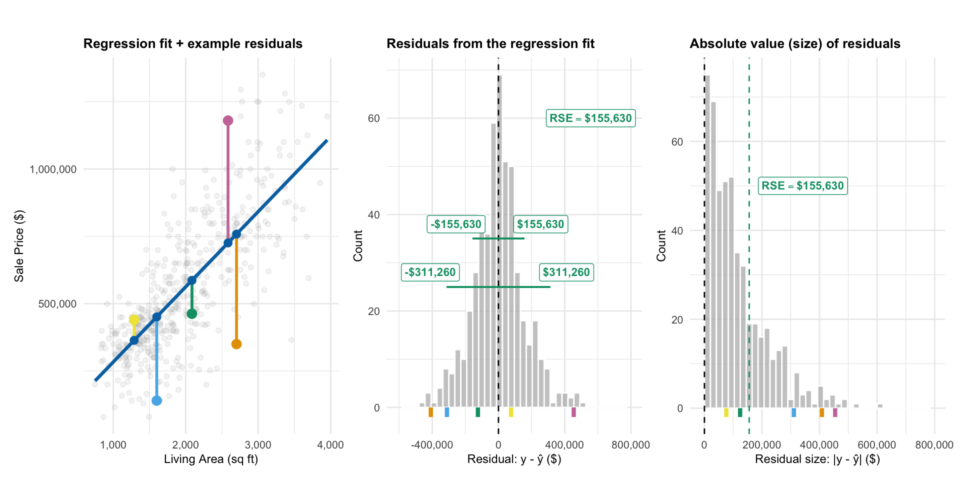
What is a “typical” residual?

The residual tells us the prediction error for a given point
The standard deviation of the residuals tells us the typical size of these prediction errors (in absolute value)
It’s a measure of how variable our prediction errors are
- Low variability: our predictions are usually close to actual values
- High variability: our predictions are often far off from actual values
In R, this is called the Residual Standard Error (RSE)

summary(fit)


Call:
lm(formula = price ~ area, data = houses)

Residuals:
    Min      1Q  Median      3Q     Max 
-604840  -90641    2955   83298  519720 

Coefficients:
             Estimate Std. Error t value            Pr(>|t|)    
(Intercept)  4296.668  21017.955  0.2044              0.8381    
area          279.139     10.101 27.6337 <0.0000000000000002 ***
---
Signif. codes:  0 '***' 0.001 '**' 0.01 '*' 0.05 '.' 0.1 ' ' 1

Residual standard error: 155630 on 506 degrees of freedom
Multiple R-squared:  0.60146,   Adjusted R-squared:  0.60067 
F-statistic: 763.62 on 1 and 506 DF,  p-value: < 0.000000000000000222

From line 16: RSE = $155,630

Another interpretation of RSE

The residuals look approximately Normally distributed
The mean of the residuals is 0
The standard deviation of the residuals is the RSE
95% of a Normal distribution is within 2 standard deviations of the mean
Therefore: 95% of the time, the prediction error is within \pm 2 \times \text{RSE} of the predicted value

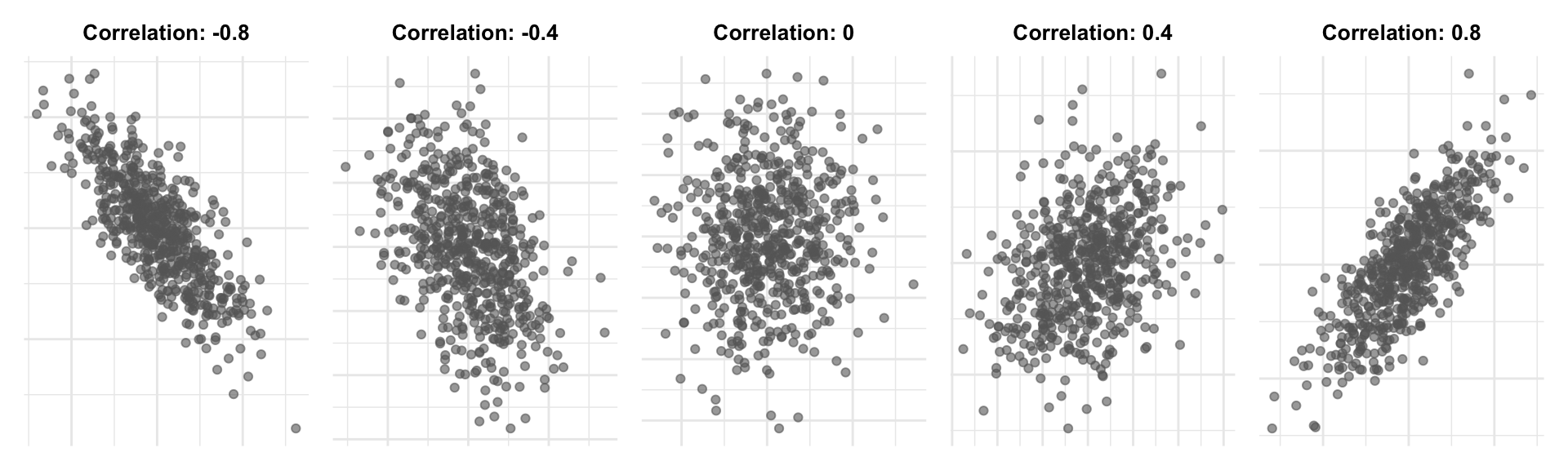
Correlation

\text{Cor}(X,Y) measures linear association between two variables

Between -1 and +1
Sign indicates direction of linear relationship
Magnitude indicates strength of linear relationship (0 = none, \pm 1 = perfect)

Correlation

R^2 (R-squared)

R^2 is a measure of the strength of the linear relationship between the Y and all X’s in the linear regression

R^2 ranges from 0 to 1
- 0 = no linear relationship
- 1 = perfect linear relationship

Defining R^2

R^2 has two equivalent definitions:

The squared correlation between observed and fitted values from the regression model
The proportion of variance in the outcome Y “explained” by the regression model

Finding R^2

summary(fit)


Call:
lm(formula = price ~ area, data = houses)

Residuals:
    Min      1Q  Median      3Q     Max 
-604840  -90641    2955   83298  519720 

Coefficients:
             Estimate Std. Error t value            Pr(>|t|)    
(Intercept)  4296.668  21017.955  0.2044              0.8381    
area          279.139     10.101 27.6337 <0.0000000000000002 ***
---
Signif. codes:  0 '***' 0.001 '**' 0.01 '*' 0.05 '.' 0.1 ' ' 1

Residual standard error: 155630 on 506 degrees of freedom
Multiple R-squared:  0.60146,   Adjusted R-squared:  0.60067 
F-statistic: 763.62 on 1 and 506 DF,  p-value: < 0.000000000000000222

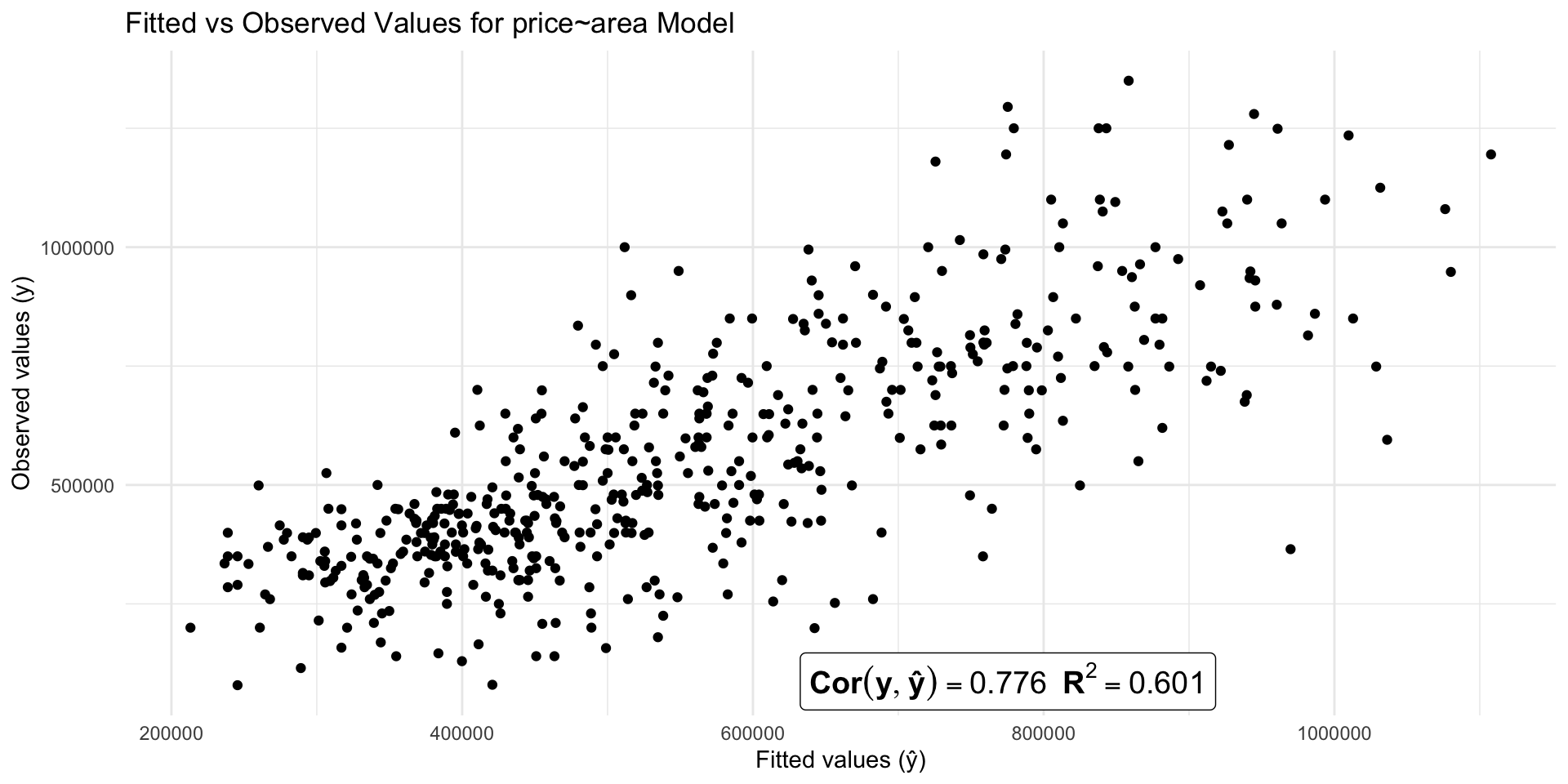
Line 17 (Multiple R-squared): R^2 = 0.601 (we’ll cover adjusted R^2 later)

R^2 = \text{Cor}(Y, \hat{Y})^2

R^2 as generalized correlation

R^2 tells us how closely the predicted values track actual values
In a simple linear model, it’s the same as \text{Cor}(X,Y)^2
So you can think of R^2 as a generalization of correlation to multiple X’s

R^2 as generalized correlation

It inherits the same limitations as correlation:

Low R^2 does not imply
- No “meaningful” linear relationship
- No strong nonlinear relationship

R^2 as generalized correlation

High R^2 does not imply
- A causal relationship
- A true linear relationship
- Prediction errors are small enough to be useful
- The model will predict well for future data

R^2 as proportion of variance “explained”

If R^2 is high then our predictions track the observed values closely
R^2 measures how much unpredictability (variance) in the outcome “goes away” when we ues X to predict

R^2 as proportion of variance “explained”

R^2 = \frac{\overbrace{\text{variance of Y} - \text{variance of residuals}}^{\text{variance ``explained''}}}{\text{variance of Y}}

Common phrasing: “R^2 is the proportion of variance in Y explained by the model”

R^2 as proportion of variance “explained”

\begin{align*} R^2 &= \frac{\overbrace{\text{variance of Y} - \text{variance of residuals}}^{\text{variance ``explained''}}}{\text{variance of Y}} \\ &= \frac{246274^2 - 155630^2}{246274^2}\approx 0.601 \end{align*}

R^2 as proportion of variance “explained”

We say X “explained” 60.1% of the total variability in Y
Remember: this is just a way of quantifying how closely the line tracks actual values
- You can predict something without being able to explain why it happens!

R^2 or RSE?

R^2 measures the strength of the linear relationship between Y and the X’s
- Since it’s a relative measure, we don’t know how big our prediction errors are likely to be
RSE measures the typical size of our prediction errors using X to predict Y
- Since it’s an absolute measure, we don’t know how strong the linear relationship is

Both can be useful, but in practice RSE is usually more relevant.

R^2 or RSE?

Predicting the price of a house from its area:

R^2 = 0.601
\text{RSE} = \$155630

Pretty strong linear relationship, but typical prediction errors are still very large!

R^2 doesn’t add up

We can use R^2 to measure “independent” contributions of multiple X variables
Compare R^2 from models with different sets of X variables
- Area: R^2 = 0.601
- Beds: R^2 = 0.137
- Area and Beds R^2 = 0.615 \neq 0.601+0.137
Adding beds once you know area explains only about 1.4% more variance!

Why?

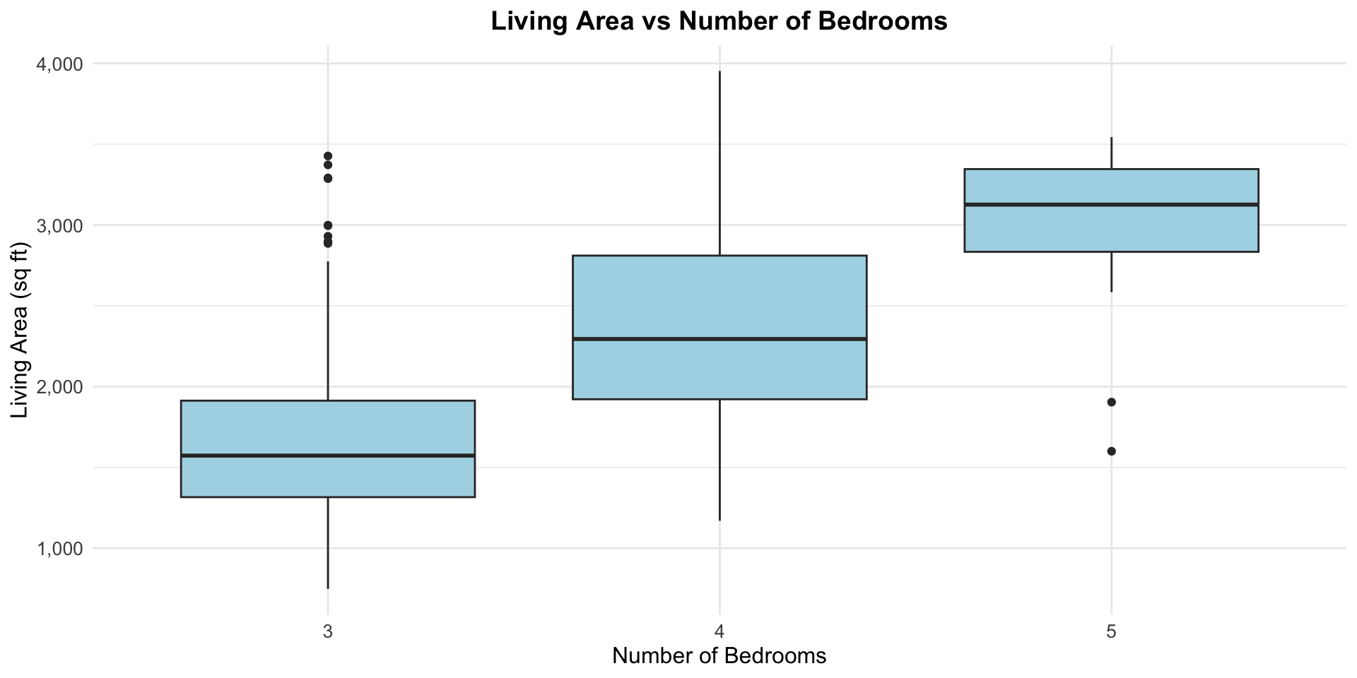
Area already contains a lot of information about beds
The new information we get from introducing beds is not that useful for predicting prices
Compare this to starting with beds and adding area – we get a big boost in R^2

Prediction isn’t everything

Notice that the area and area+beds model have very similar R^2 values
The RSE values are also similar
- Area only: 155627
- Area + Beds: 153047
Both models predict prices about equally well (or badly)
- But they tell very different stories about what an additional sqft is worth!

Incorporating uncertainty

What personal characteristics about an instructor do you think are predictive of the scores they receive on student evaluations?

Hamermesh & Parker (2005) data set

Student evaluations of N=463 instructors at UT Austin, 2000-2002
For each instructor:
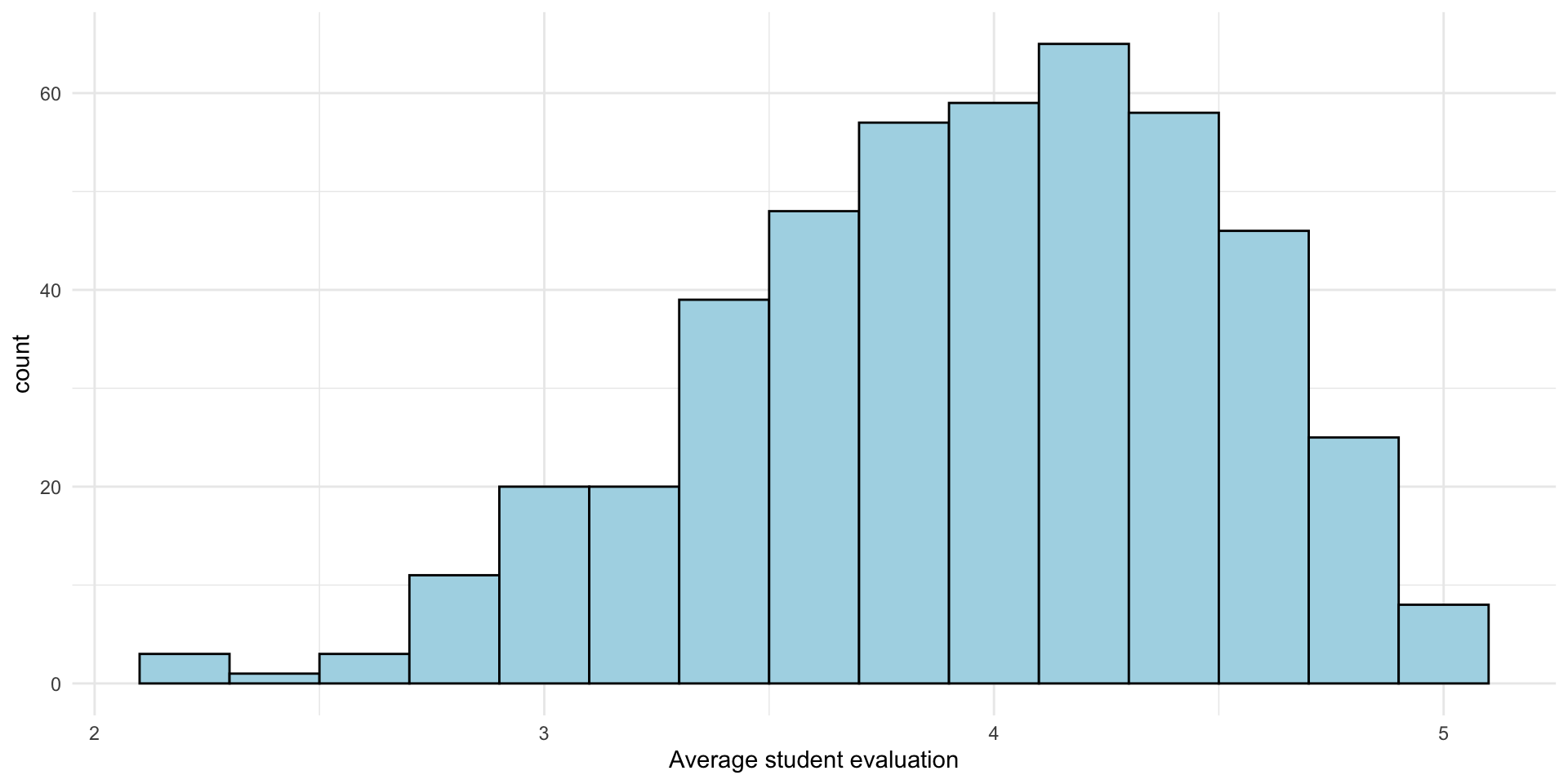
- eval: average student evaluation of teacher
- beauty: average beauty score from a six-student panel (z-score, 0 is average)
- gender: male or female
- credits: single- or multi-credit course
- age: age of instructor
- (and more…)

Explore the data: `eval`

Explore the data: `beauty`

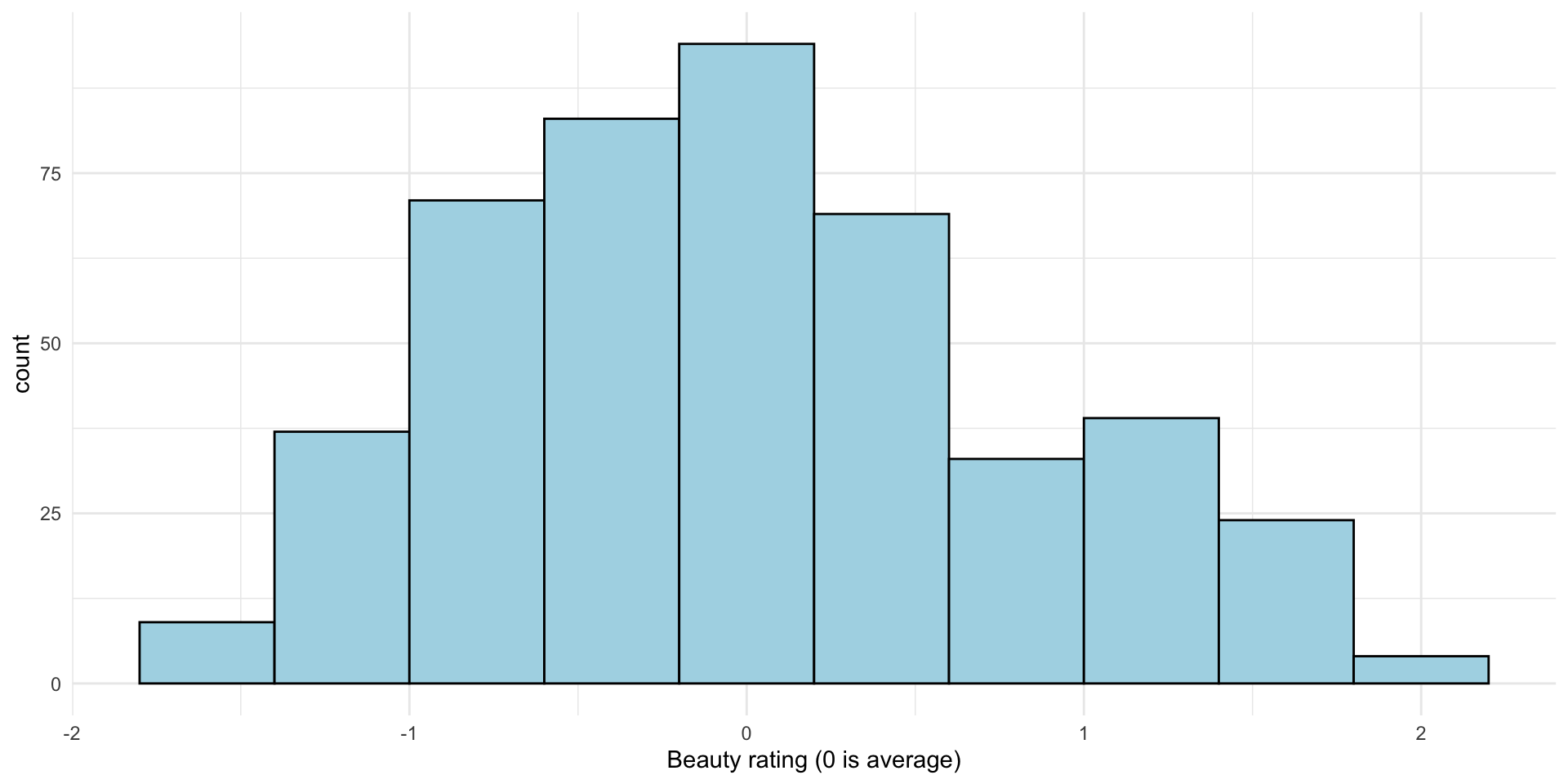
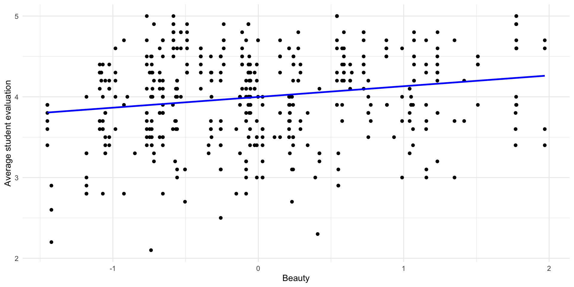
Do you think there is a positive or negative relationship between beauty and evaluations?

The simple regression fit

model2 <- lm(eval ~ beauty, data = profs)
summary(model2)


Call:
lm(formula = eval ~ beauty, data = profs)

Residuals:
    Min      1Q  Median      3Q     Max 
-1.8002 -0.3630  0.0725  0.4021  1.1037 

Coefficients:
            Estimate Std. Error t value             Pr(>|t|)    
(Intercept)   3.9983     0.0253  157.73 < 0.0000000000000002 ***
beauty        0.1330     0.0322    4.13             0.000042 ***
---
Signif. codes:  0 '***' 0.001 '**' 0.01 '*' 0.05 '.' 0.1 ' ' 1

Residual standard error: 0.545 on 461 degrees of freedom
Multiple R-squared:  0.0357,    Adjusted R-squared:  0.0336 
F-statistic: 17.1 on 1 and 461 DF,  p-value: 0.0000425

The simple regression fit

Accounting for error and uncertainty

So far we’ve focused on estimated coefficients and predictions
But we only have a sample of instructors – what would the regression line look like if we had the entire population of all instructors in the world?
We know our predictions will be wrong – how wrong are the likely to be?
We know our coefficients don’t match the true population values – how close are they?

The simple linear regression model

We need a model for our data to answer these questions. Our model has four components:

Linearity
Independence of prediction errors
Normality of prediction errors
Equal variance of prediction errors

Linearity

The relationship between Y and each X is linear:

Y = \beta_0 + \beta_1 X_{1} + \beta_2 X_{2} + ... + \beta_p X_{p} + \epsilon

\beta_0, \beta_1, ..., \beta_p are the true/population regression coefficients
\epsilon is the true error if we predict Y using the true regression coefficients

Our other assumptions are about those true error terms \epsilon…

Independence

Each observation has an independent true error term
If my neighbor’s house sells for more than expected, that doesn’t tell me anything about whether my house will sell for more or less than expected
If the last house sells for less than expected, that doesn’t tell us anything about whether the next house will sell for more or less than expected

Normality

The true error terms \epsilon are normally distributed and centered at zero

The average error over many predictions is zero
Over-prediction and under-prediction are equally likely
Most errors are small, but large errors are possible

Equal Variance

The size of the true errors does not depend on the values of the X’s (or anything else)
- For example, errors are about the same size (on average) for small and large houses

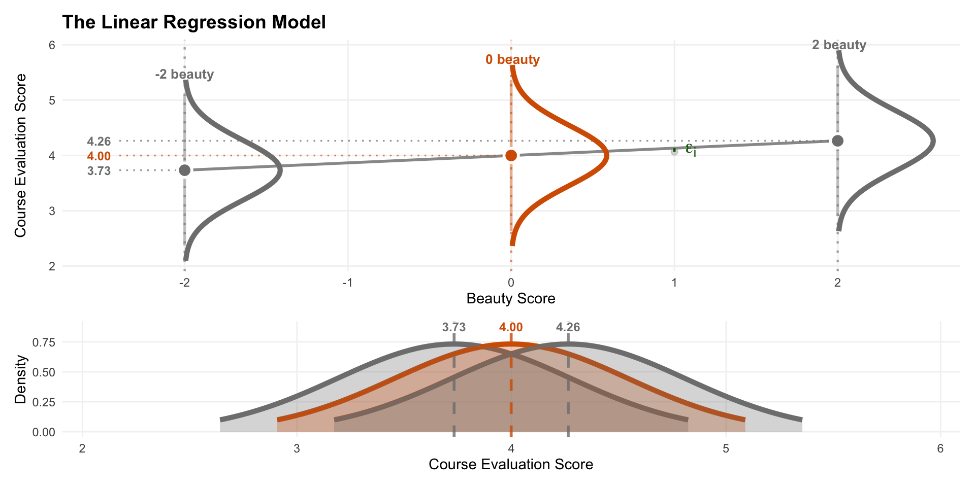
Visualizing the linear model

Estimates vs True Values

Our \hat \beta_0, \hat \beta_1, ..., \hat \beta_p are just estimates of the true \beta_0, \beta_1, ..., \beta_p
The residuals estimate the true prediction errors
The RSE (standard deviation of residuals) is an estimate of the true \sigma (error standard deviation)

Accounting for uncertainty in estimates

If we want to know how uncertain our estimates are, we need to quantify their variability.
We can do this using the sampling distribution of our estimates (how much they change over repeated samples)
More specifically, we can compute confidence intervals

Confidence intervals

A confidence interval gives a range of plausible values for a population parameter (e.g., a regression coefficient)
These are possible values of the true coefficients that are consistent with our observed data at a given level of confidence (e.g., 95%)
If our LINE assumptions hold, these are easy to get:

confint(model2)

             2.5 % 97.5 %
(Intercept) 3.9485  4.048
beauty      0.0698  0.196

Is there evidence for a linear relationship?

confint(model2)

             2.5 % 97.5 %
(Intercept) 3.9485  4.048
beauty      0.0698  0.196

The range of plausible values for the slope \beta_1 is (0.07, 0.20)
No linear relationship would mean \beta_1=0
All the plausible values are positive, so we have statistically significant evidence of a positive linear relationship between beauty and evaluations

How strong is the linear relationship?

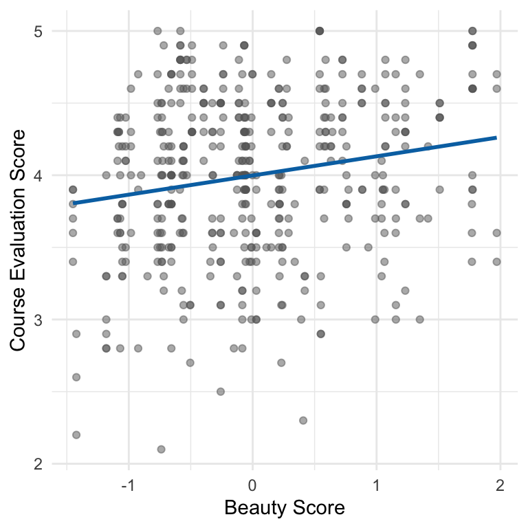
\text{Cor}(\text{beauty}, \text{eval}) = 0.19
R^2 = 0.036 – only 3.6% of the variance in eval is explained by beauty
But we have strong statistical evidence that this (weak) linear relationship holds among the population of all instructors
- i.e., it isn’t just a fluke in this particular sample

How strong is the linear relationship?

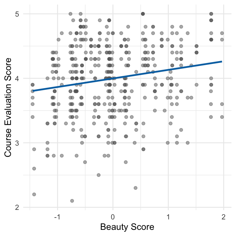
Remember: R^2 doesn’t tell us directly how confident we are that a linear relationship exists
In this case we have strong evidence of a weak linear relationship
This is because many factors unrelated to beauty affect eval scores

Accounting for uncertainty in predictions

If I’m trying to predict the evaluation score of a particular professor’s course, I’d like to know:

What’s the most likely evaluation score (best prediction)?
What’s a range of likely evaluation scores (prediction interval) – because my prediction will almost certainly be wrong!

Prediction intervals

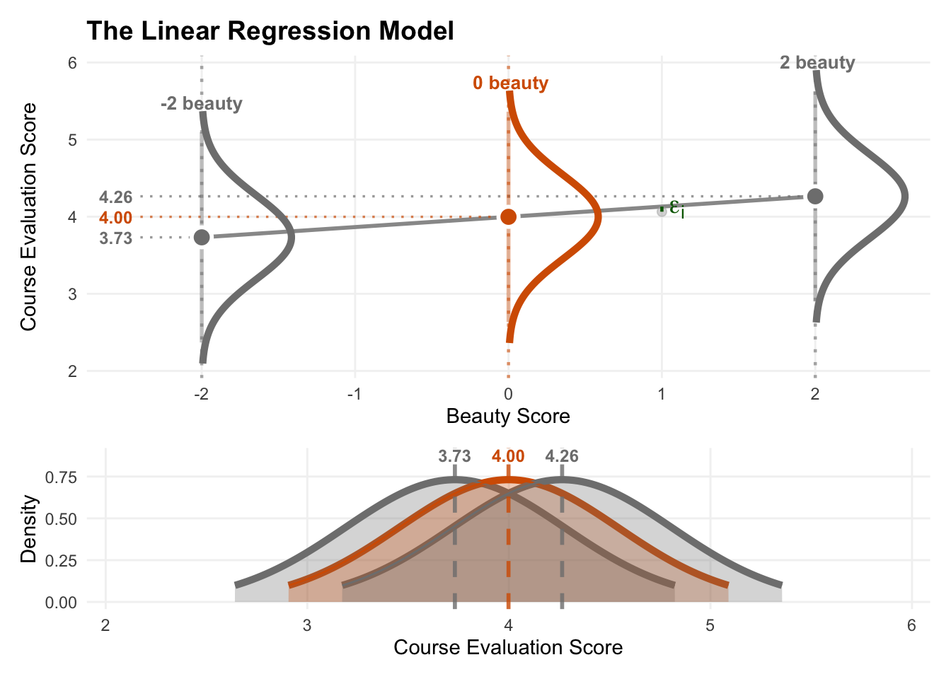
Our model: Actual evaluation scores for professors of a given beauty score will:

Have normal distributions
Centered at the predicted value (location on the line)
With standard deviation \sigma

95% of the time, actual prices fall within \pm 2\sigma of the predicted price (if we knew the true line and \sigma)

Prediction intervals

Under our LINE assumptions, we can get prediction intervals for new observations that account for both:

Uncertainty in our estimated regression line
The inherent variability in actual outcomes around that line

For a fairly ugly professor (beauty score = -1), we predict an evaluation score of:

predict(model2, list(beauty = -1), interval = "prediction")

   fit  lwr  upr
1 3.87 2.79 4.94

We can be 95% confident that the actual evaluation score for this professor will fall between 2.79 and 4.94.

Error, Uncertainty and the Linear Model

Posit Cloud vs RStudio

Measuring prediction error

Predicting price from area

Residuals and fitted values

Visualizing residuals and fitted values

What does a residual tell us?

What is a “typical” residual?

Another interpretation of RSE

Correlation

Correlation

R^2 (R-squared)

Defining R^2

Finding R^2

R^2 = \text{Cor}(Y, \hat{Y})^2

R^2 as generalized correlation

R^2 as generalized correlation

R^2 as generalized correlation

R^2 as proportion of variance “explained”

R^2 as proportion of variance “explained”

R^2 as proportion of variance “explained”

R^2 as proportion of variance “explained”

R^2 or RSE?

R^2 or RSE?

R^2 doesn’t add up

Why?

Prediction isn’t everything

Incorporating uncertainty

Hamermesh & Parker (2005) data set

Explore the data: eval

Explore the data: beauty

The simple regression fit

The simple regression fit

Accounting for error and uncertainty

The simple linear regression model

Linearity

Independence

Normality

Equal Variance

Visualizing the linear model

Estimates vs True Values

Accounting for uncertainty in estimates

Confidence intervals

Is there evidence for a linear relationship?

How strong is the linear relationship?

How strong is the linear relationship?

Accounting for uncertainty in predictions

Prediction intervals

Prediction intervals

Explore the data: `eval`

Explore the data: `beauty`