Data Science for Business Applications

Class 11 - Random Forest

Review on Decision Trees

• What kinds of models do we know how to make?
• Classification or Regression
• We can use decision trees for either kind of \(Y\) variable.

Pros & Cons of Decision Trees

• Main Advantages:
  • Easy to interpret and explain (you can plot them!)
  • Mirrors human decision-making
  • Can handle qualitative predictors (without need for dummies)
• Main disadvantages:
  • Accuracy not as high as other methods
  • Very sensitive to training data (e.g. overfitting)
  • Biased toward dominant classes

What we can do to improve?

• Improve accuracy?

• Less sensitive to random changes in the data?

• More relevance for low-frequency classifications?

• Solution: Bagging - Bootstrap Aggregation

  • Bootstrap - quantify sampling variability by resampling from the sample.
  • In Bagginig we basically we use bootstrap on the data and then we aggregate the results.

Bootstrap & Resampling

• Sampling with replacement: each case selected for the sample is then replaced.

• Every bootstrapped sample may have its own pattern of ties and omissions.

Bagging

• Aggregate the results from the method applied to each bootstrap sample.
• This is also known as an ensemble, or combining the results of multiple models.

Bagging & Ensembling

• You want to predict on new test data.
• For classification, take the majority vote!
• For regression, take the mean or mode!

Random Forests

• Random sampling of my training data rows helps to reduce variation in my predictions that are due to randomness.

• We saw last week: sometimes the importance of individual variables can change from dataset to dataset, and therefore from model to model.

• What if we random sample the columns (variables) as well as the rows?

Random Forests

• Considering the Titanic data

• We again predict if the passenger survived (yes, no) - Categorical Variable

• Classification model

• Before, I had sex as the variable defining the first split.

• In my new trees, what if I only give the option for passengerClass and adult?

Random Forests

Let’s build a Random Forest (RF) in R

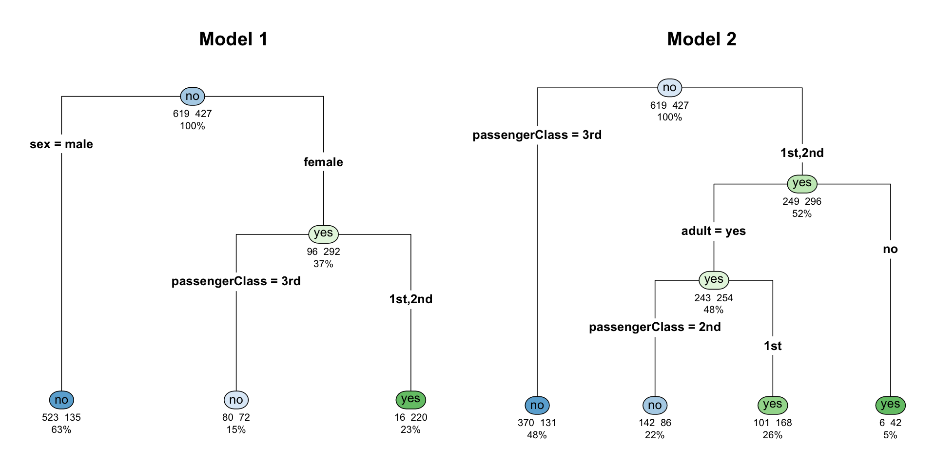
library(randomForest)
# Run the model
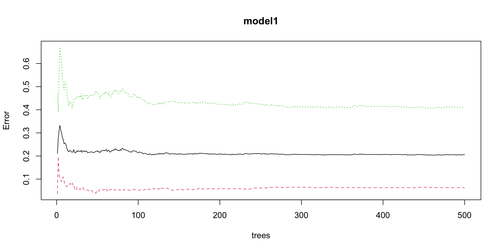
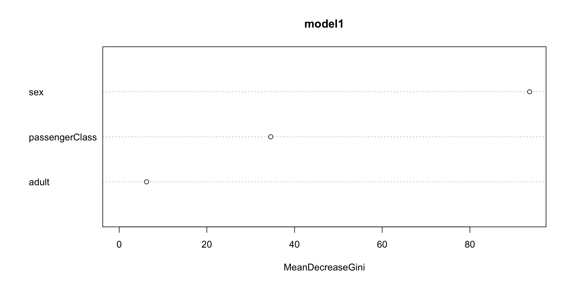
model1 = randomForest(survived ~ adult + sex + passengerClass, data = titanic_age)
# Show details on the model
print(model1)

Call:
 randomForest(formula = survived ~ adult + sex + passengerClass,      data = titanic_age) 
               Type of random forest: classification
                     Number of trees: 500
No. of variables tried at each split: 1

        OOB estimate of  error rate: 20.55%
Confusion matrix:
     no yes class.error
no  580  39  0.06300485
yes 176 251  0.41217799

• In an instant, we built 500 trees.
• We only had 3 variables, so the RF only needed to try one at each split, and grow the tree.
• OOB (Out-of-Bag) error rate: 20.46%
• (580+252)/1046 = 0.795

Classification Error estimates

plot(model1)

• The plot shows how the error change given more trees are generated.
  • OOB (black line)
  • Among passengers who did not survive, the error in prediction (red line)
  • Among passengers who did survive, the error in prediction (green line)

Feature Importance

• Feature (or variable) importance is an output from random forests.
• In this case sex was by far most helpful as the first divide in the trees.
• Adult was the least important variable in terms of predicting survival.

importance(model1)

               MeanDecreaseGini
adult                  6.241061
sex                   93.624871
passengerClass        34.567394

• The Mean Decrease in Gini: measures how much each variable contributes to reducing uncertainty when the trees are built in the random forest.

• A higher value means the variable is more important for making accurate classifications.

Feature Importance

• The importance of the variable on the split can also be displayed in a plot.

varImpPlot(model1, sort = TRUE)

Random Forest for Regression

• In this model we’ll now predict the Age of the passengers given class, gender, if they survived or not.

# Run the model
model2 = randomForest(age ~ sex + passengerClass + survived, data = titanic_age)
# Show details on the model
print(model2)

Call:
 randomForest(formula = age ~ sex + passengerClass + survived,      data = titanic_age) 
               Type of random forest: regression
                     Number of trees: 500
No. of variables tried at each split: 1

          Mean of squared residuals: 172.4933
                    % Var explained: 16.89

• The MSE is given by 173.036, or RMSE = \(\sqrt{173.036}\) = 13.15
• Variation explained 16.63 (similar to the \(R^2\))

Regression Error estimates

• The plot displays the MSE in relation to the number of trees generated.

plot(model2)

Random Forest for Regression

• Variance importance for this model

varImpPlot(model2, sort = TRUE)

Take aways of the Random Forests

• Improve accuracy on new data

• Less sensitive to random changes in the data.

• More relevance for low-frequency classifications.

• Random forests give me a lot of the benefit of decision

• trees with fewer downsides!