Data where the cases represent time: data collected every day, month, year, etc.
Time series are important for both explaining how variables change over time and forecasting the future
Examples of time series data:
Google’s closing daily stock price every day in 2020
Inventory levels of each item at a retail store at the end of every week in 2020
Number of new COVID cases in the US each day since the start of the pandemic
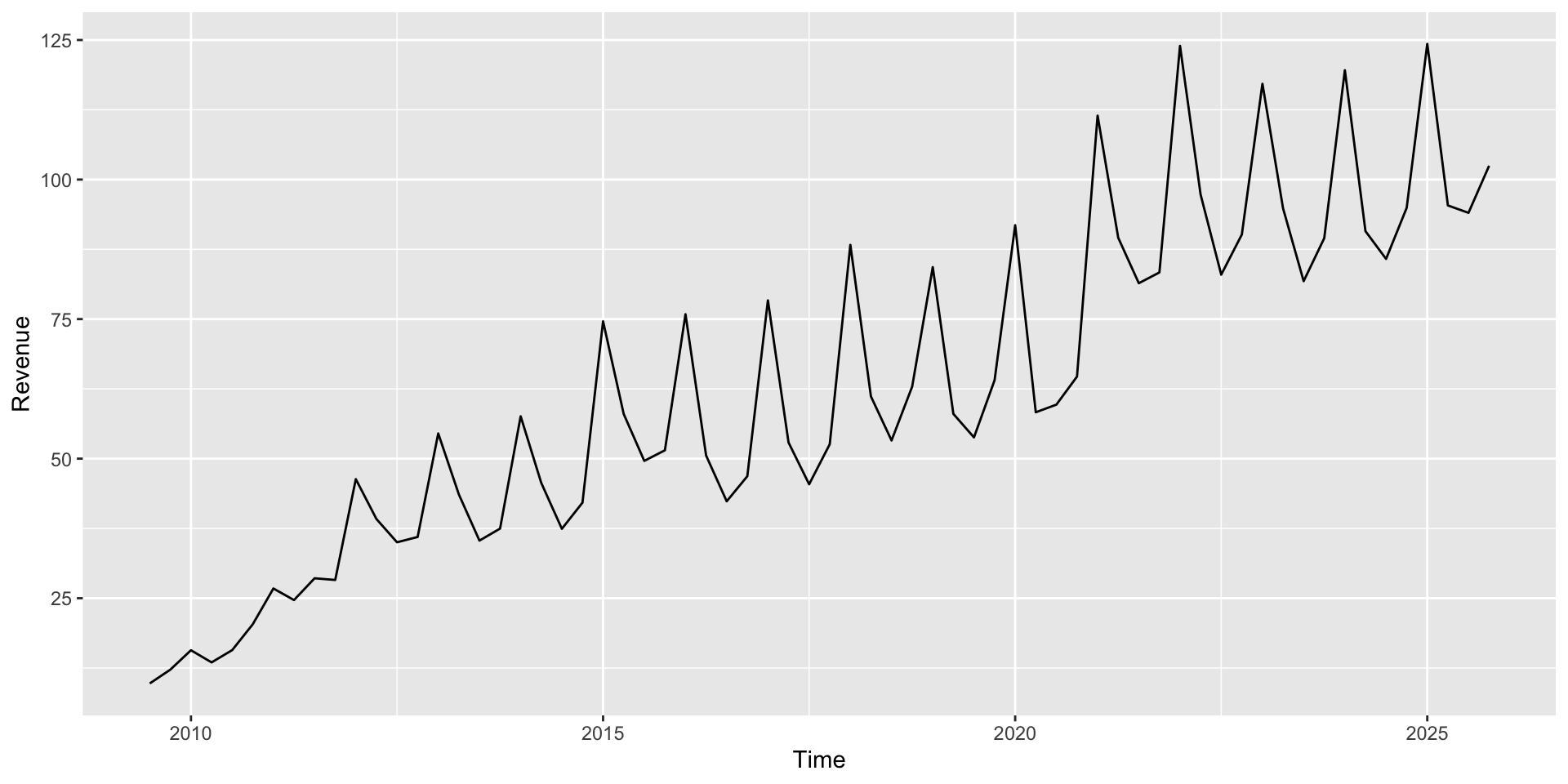
Apple’s quarterly revenue since 2009
Anatomy of a time series
Some notation:
\(t = 1,2,3,...\), time index
\(Y_t\), is the value: of the variable of interest at time \(t\)
\(Y_t\) may be composed of one or more components:
Trend
Seasonal
Cyclical
Random
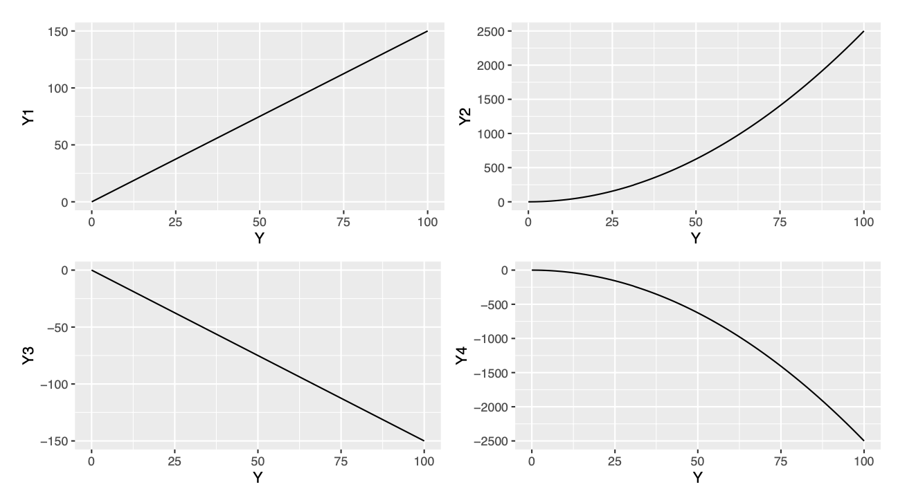
Trend component
A trend is persistent upwards or downwards movement in the data (not necessarily linear).
Trend component
Example: Moore’s Law (accelerating increase of transistor count)
Example: US population over time
A time series with no trend is called stationary.
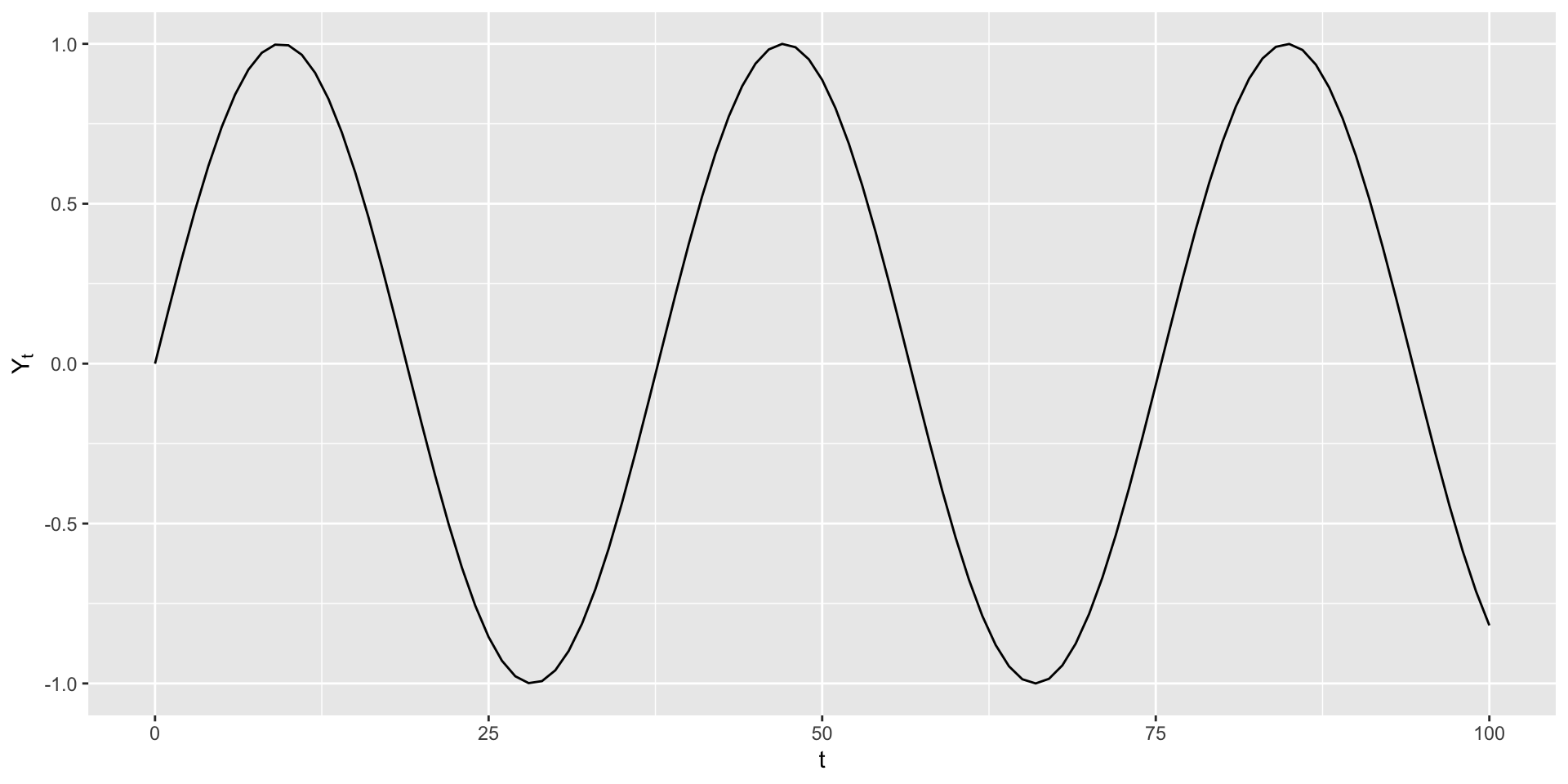
Seasonal component
Seasonal fluctuation occurs when predictable up or down movements occur over a regular interval.
Seasonal component
The ups and downs must occur over a regular interval (e.g., every month, or every year)
Example: Highway traffic volume is highest during rush hour every day
Example: Supermarket sales may be highest every month right after common paydays like the 15th and 30th
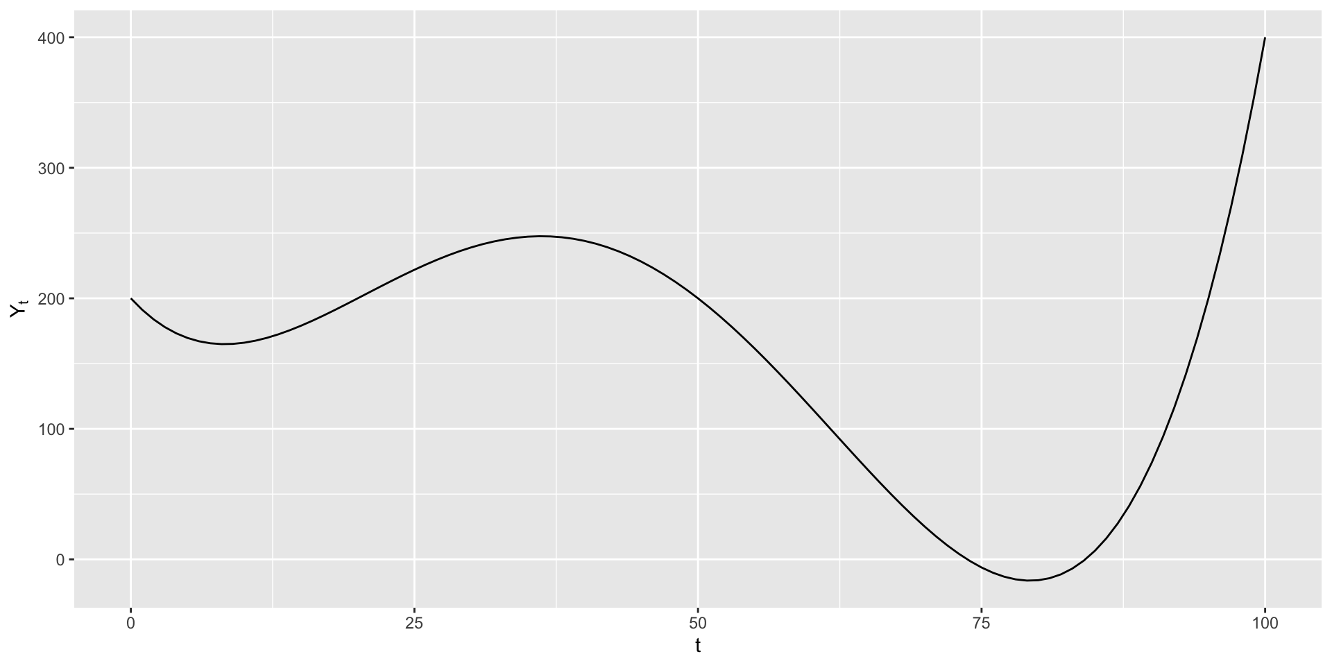
Cyclic component
Cyclic fluctuations occur at unpredictable intervals, e.g. due to changing business or economic conditions.
Cyclic component
In contrast to seasonal fluctuations, cyclic fluctuations do not occur at regular, predictable intervals
It may be possible to predict cyclic components based on some other (non-time) variable
Example: Restaurant sales dropped dramatically in 2020 due to COVID, as people ate out less
Example: Sales of bell bottoms rose in the 60s and 70s, declined by the 80s, and then had a resurgence in the 90s
Remainder/Error component
Any real time series will always have random noise as well, which can’t be predicted or forecast.
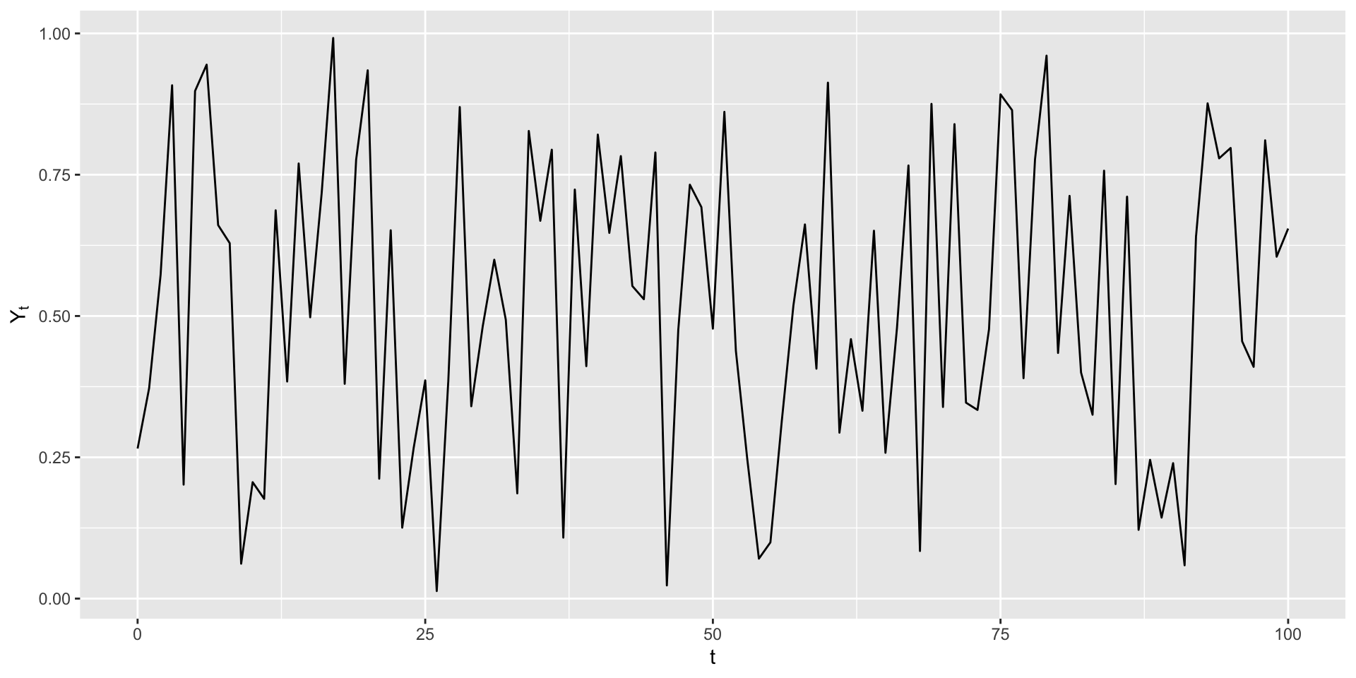
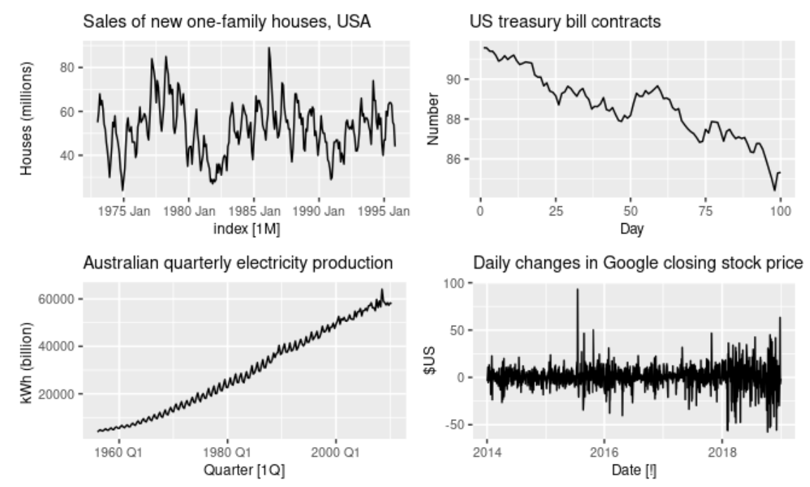
Time Series Components
Which component(s) you see in each of these time series?
Putting these together
Real time series will usually include a combination of these four components. We will model the time series \(Y_t\) either additively:
\[
Y_t = \text{Trend} + \text{Seasonal} + \text{Random} = T_t +S_t +E_t
\] Or multiplicatively: \[
Y_t = \text{Trend}\cdot\text{Seasonal}\cdot\text{Random}= T_t \cdot S_t \cdot E_t
\] * (\(E_t\) consists of both the cyclic and error components, as both are unpredictable.) This model can be rewritten as a log model: \[
\log{Y_t} = \log(T_t) + \log(S_t) + \log(E_t)
\]
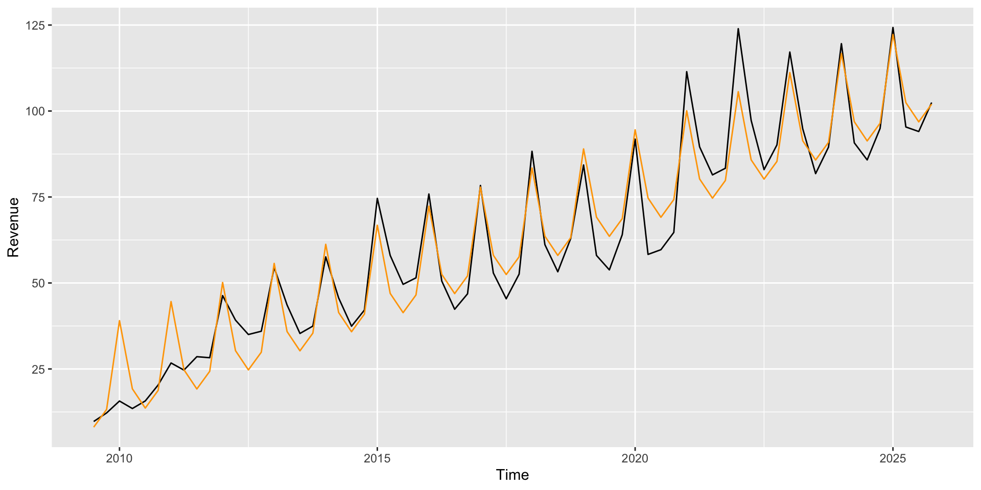
What does the final model predict from the Quarter component indicates: for Apple in 2030 Q1? (Should we trust that prediction?)
Fitting an Additive model
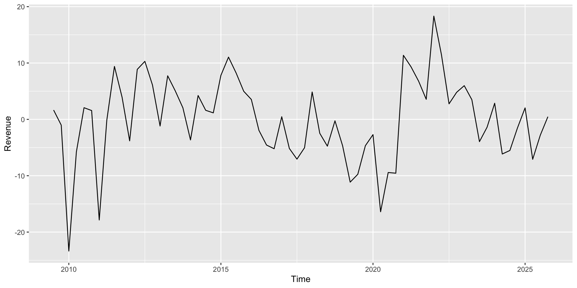
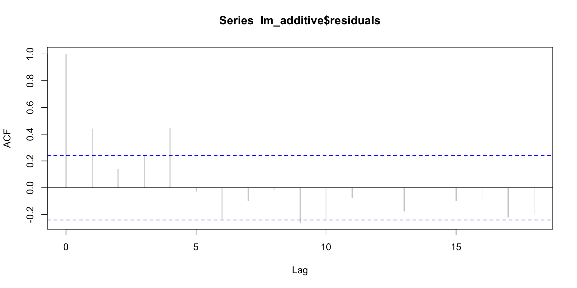
The residuals from this model show the “detrended and deasonalized” data (but there’s still some trend left!):
We hadn’t yet dealt with the time dependence
ggplot(apple, aes(x = Time, y = Revenue)) +geom_line(aes(x = Time, y =residuals(lm_additive)))
Autorgression model
How we deal with the time dependence ? Key idea: Instead of predicting \(Y_t\) as a function of \(t\) (or other variables), predict \(Y_t\) as a function of \(Y_{t-1}\): \[
Y_t = \beta_0 + \beta_1 Y_{t-1} + e_t
\]
\(Y_{t-1}\) is called the “1st lag” of \(Y\)
This is called autoregressive (AR) because it predicts the values of a time series based on previous values
The model above is an AR(1) model
We can have AR(\(p\)) models, with lag \(p\)
Autocorrelation
Autocorrelation, is the correlation of \(Y_t\) with each of its lags \(Y_t, Y_{t−1},\dots\)\[
Cor(Y_t, Y_{t−1}), Cor(Y_t, Y_{t−2}),\dots
\]
We also have the autocorrelation of the residuals, \(r_t\)’s, which indicates that there’s a strong indication that the independence assumption is violated \[
Cor(r_t, r_{t−1}), Cor(r_t, r_{t−2}),\dots
\]
Ozone example
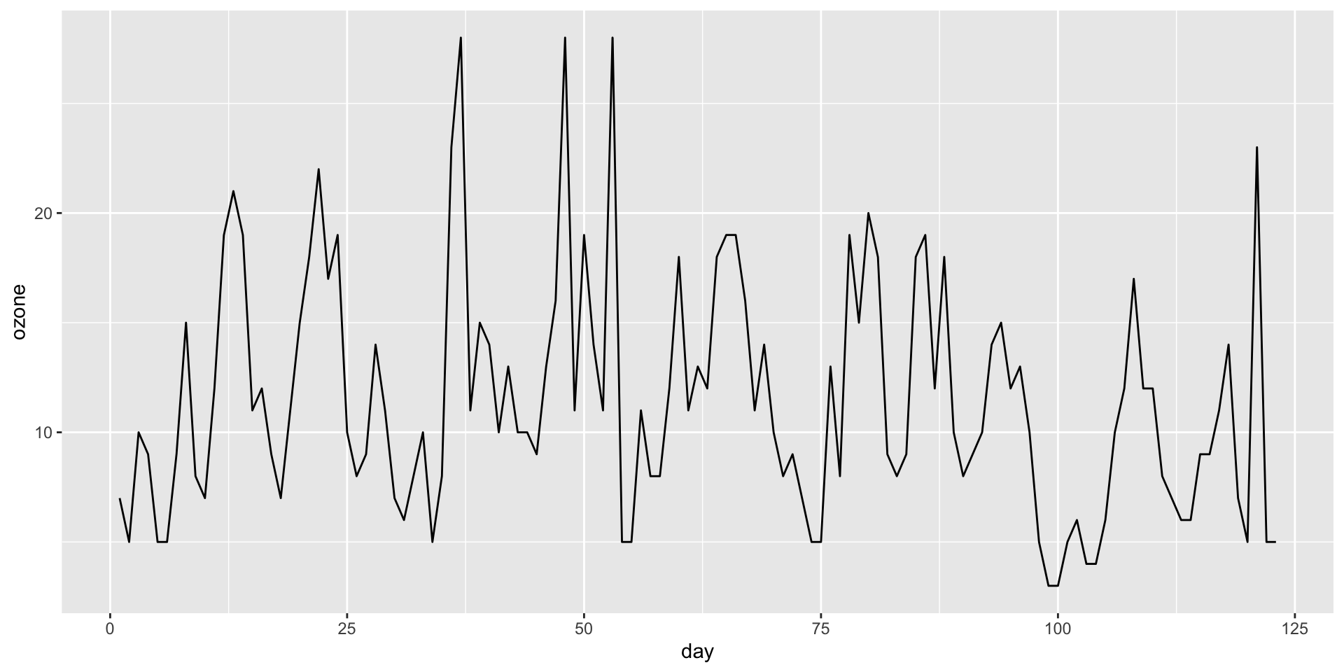
Creating an AR(1) model: Daily ozone levels in Houston
ggplot(ozone, aes(x = day, y = ozone)) +geom_line()
ACF plot
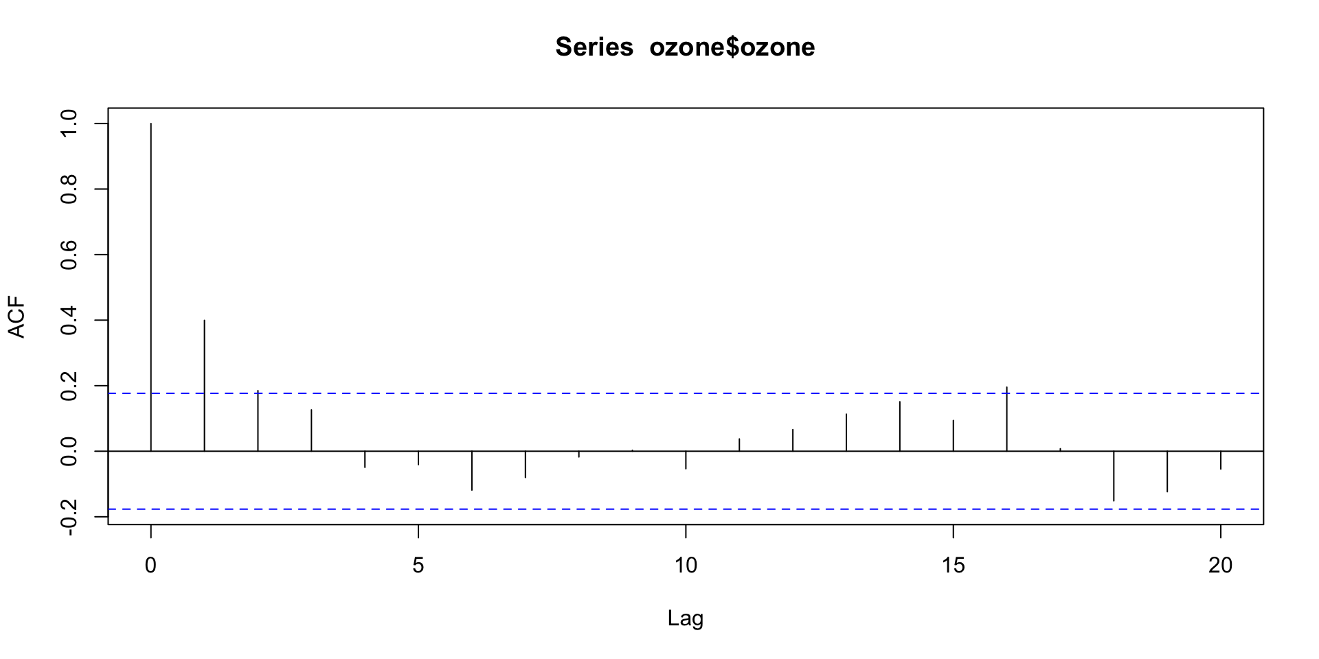
Visualizing the autocorrelation function (ACF)
acf(ozone$ozone)
Autocorrelations outside of the dashed blue lines are statistically significant.
Autorgression of the model
We use the lag function to create the lagged observations
Call:
lm(formula = ozone ~ lag1, data = ozone)

Residuals:
    Min      1Q  Median      3Q     Max
-13.192  -3.464  -1.108   2.679  16.679

Coefficients:
            Estimate Std. Error t value      Pr(>|t|)
(Intercept)  6.87446    1.06976   6.426 0.00000000276 ***
lag1         0.40419    0.08381   4.823 0.00000419740 ***
---
Signif. codes:  0 '***' 0.001 '**' 0.01 '*' 0.05 '.' 0.1 ' ' 1

Residual standard error: 4.999 on 120 degrees of freedom
  (1 observation deleted due to missingness)
Multiple R-squared:  0.1624,    Adjusted R-squared:  0.1554
F-statistic: 23.26 on 1 and 120 DF,  p-value: 0.000004197
Assumptions of an AR(1) model
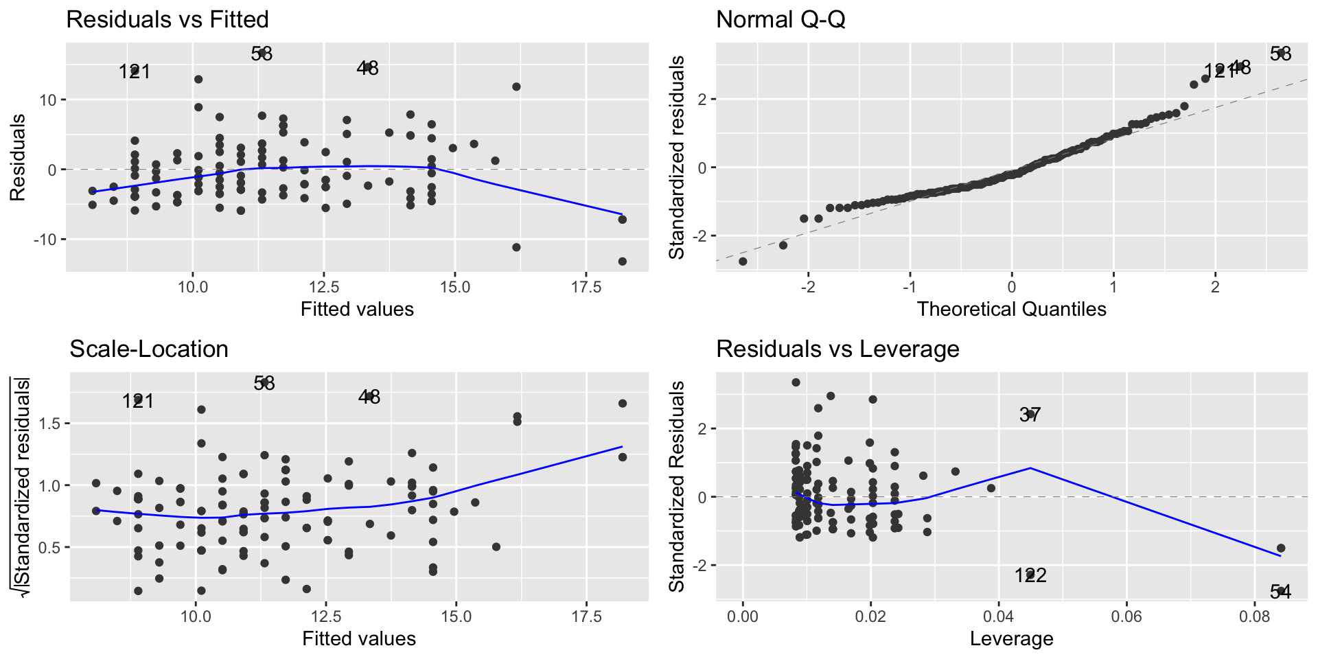
Linearity, Normality, Equal Variance: Check using residual plot (linearity + homoscedasticity), Q-Q plot (normality), scale/location (homoscedasticity) like any other regression model
Independence: Since this is a time series, we can actually check this by looking at the autocorrelation of the residuals (we want no significant autocorrelation)
Autoplot
Linearity, Normality, Equal Variance
autoplot(ozone.model)
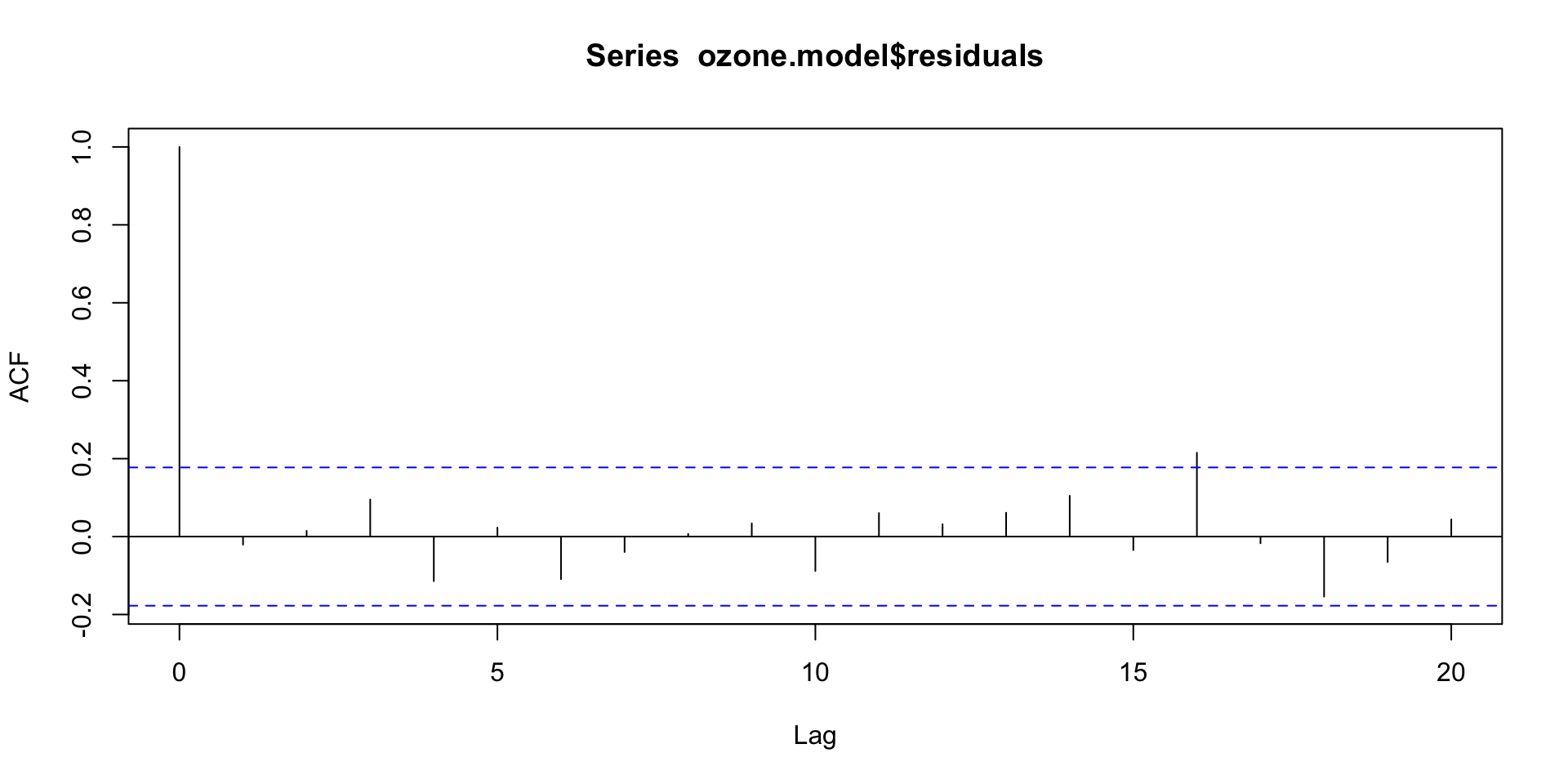
ACF of the residuals
acf(ozone.model$residuals)
We expect 5% of autocorrelations to be significant just by chance, so having just 1 out of the 20 lags flagged as significant indicates we are OK on independence!
Making predictions in time series
Type
Model
Predicted \(Y_t\)
White noise
\(Y_t = e_t\)
\(0\)
Random sample
\(Y_t = \beta_0 + e_t\)
\(\widehat{\beta}_0\) (or average \(Y\))
Random walk
\(Y_t = \beta_0 + Y_{t-1} + e_t\)
\(\widehat{\beta}_0 + Y_{t-1}\)
General AR(1)
\(Y_t = \beta_0 + \beta_1 Y_{t-1} + e_t\)
\(\widehat{\beta}_0 + \widehat{\beta}_1 Y_{t-1}\)
Unit root occurs when \(\beta_1 = 1\). This means:
The series is a random walk.
There’s no mean reversion, and any shocks will have a permanent effect.
When \(\beta_1 = 1\), the model is non-stationary, meaning the series tends to “drift” without stabilizing around a fixed mean.
If \(|\beta_1| < 1\), the series is mean-reverting, and shocks are temporary.
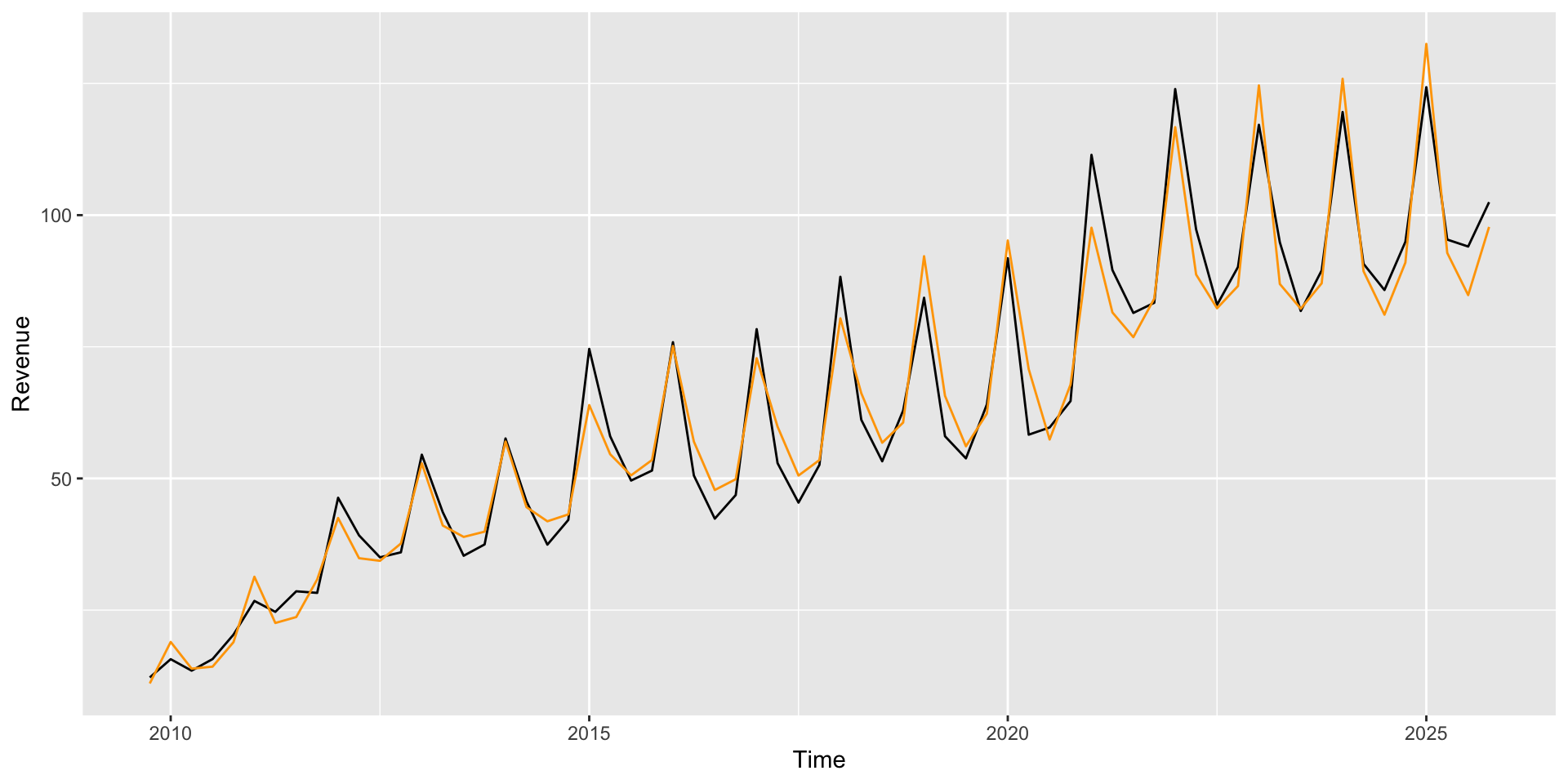
The slope associated with lag is statistically significant, and its value is between minus and plus one; we have that this is a mean-reverting time series.
We also have a better fit (here we feed lag1 with prediction from the previous period, US$ 102.47 billions):
The confidence interval for the forecast is narrower, and the difference between what we observe and predict is smaller.
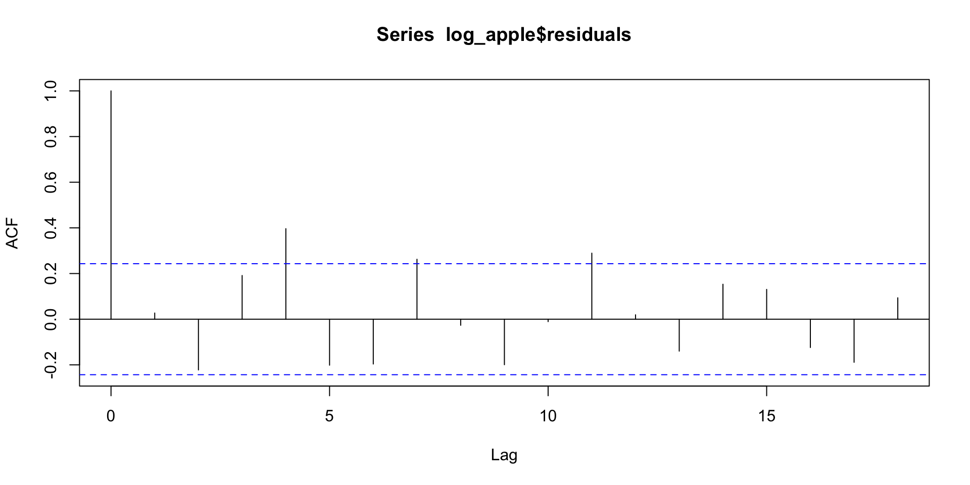
Apple Revenue ACF plot
ACF plot of the residuals of the multiplicative model.
The independent assumptions look better, but it might be necessary to add more lags.
Time Series Strategy
To building a time series model:
Start with a an additive or multiplicative model with trend and seasonal components. (Plot your data! If the seasonal variation increases or decreases over time you’ll want a multiplicative model.)
Examine the usual diagnostic plots, and plot your residuals as a function of time. Do you need a (different) nonlinear time trend? A transformation of \(Y\)?
Check your residuals for autocorrelation. If it’s present, add appropriate lag terms to your model.