Call:
lm(formula = vote02 ~ treatment, data = GOTV)

Residuals:
   Min     1Q Median     3Q    Max
-0.588 -0.546  0.454  0.454  0.454

Coefficients:
                    Estimate Std. Error t value            Pr(>|t|)
(Intercept)        0.5460484  0.0008192 666.527 <0.0000000000000002 ***
treatmenttreatment 0.0419122  0.0046177   9.076 <0.0000000000000002 ***
---
Signif. codes:  0 '***' 0.001 '**' 0.01 '*' 0.05 '.' 0.1 ' ' 1

Residual standard error: 0.4977 on 381060 degrees of freedom
Multiple R-squared:  0.0002161, Adjusted R-squared:  0.0002135
F-statistic: 82.38 on 1 and 381060 DF, p-value: < 0.00000000000000022Data Science for Business Applications
Class 10 - Randomized Control Trials
Causal Conclusion
If we run a regression predicting \(Y\) from \(X\) and find that \(X\) is a significant predictor of \(Y\), we would like to conclude that \(X\) causes \(Y\). But it might be the case that:
\(Y\) actually causes \(X\).
\(X\) and \(Y\) are not actually related in the population; they happen to be correlated in the sample just by chance.
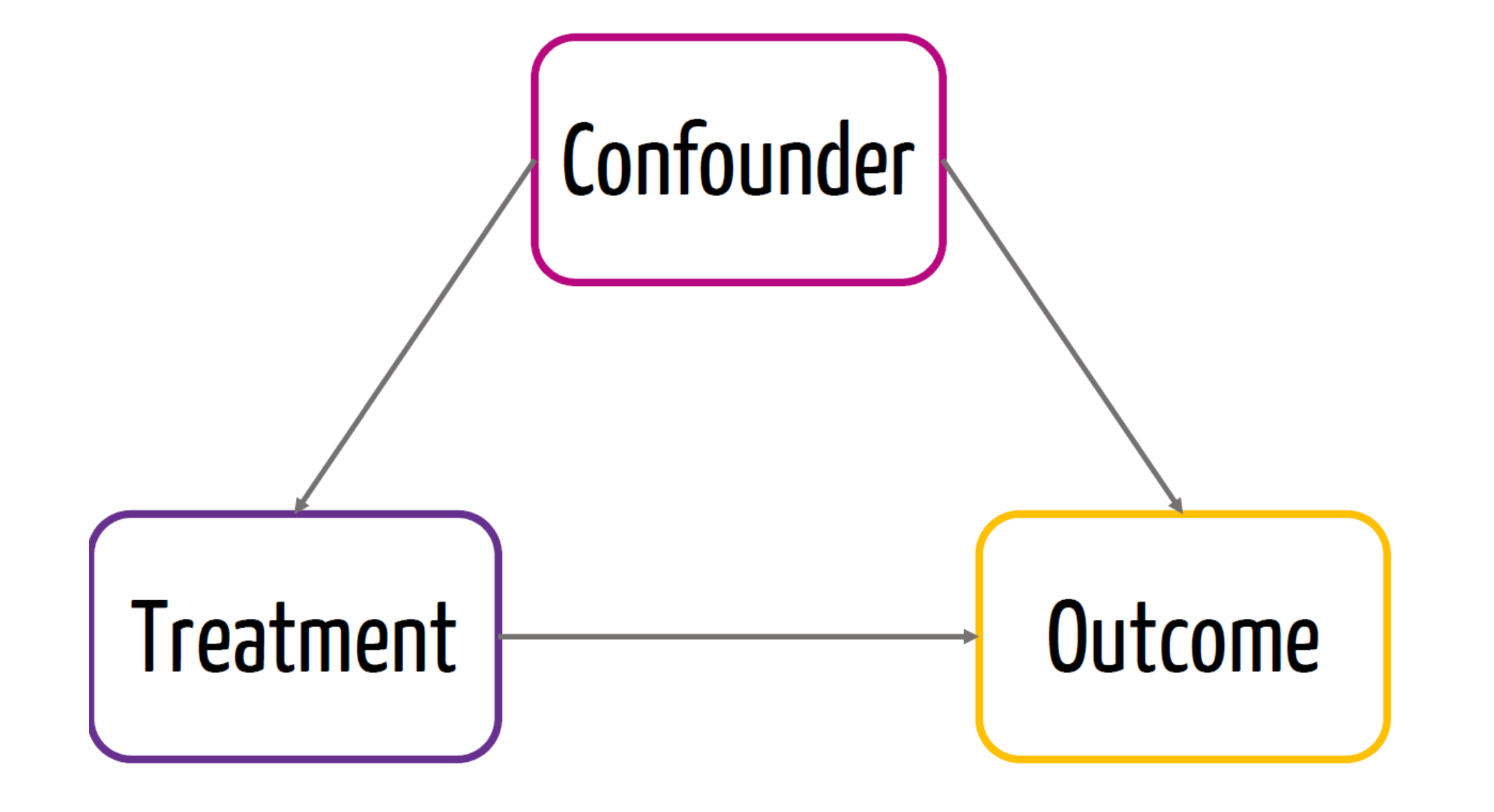
A common variable \(Z\) (a confounder) causes both \(X\) and \(Y\).
A common variable \(W\) (a collider) is caused by both \(X\) and \(Y\).
Confounders and Colliders
A confounder is a third variable that causes both \(X\) and \(Y\) and explains the observed correlation between X and Y.
A collider is a third variable that is caused by both \(X\) and \(Y\).
Randomization
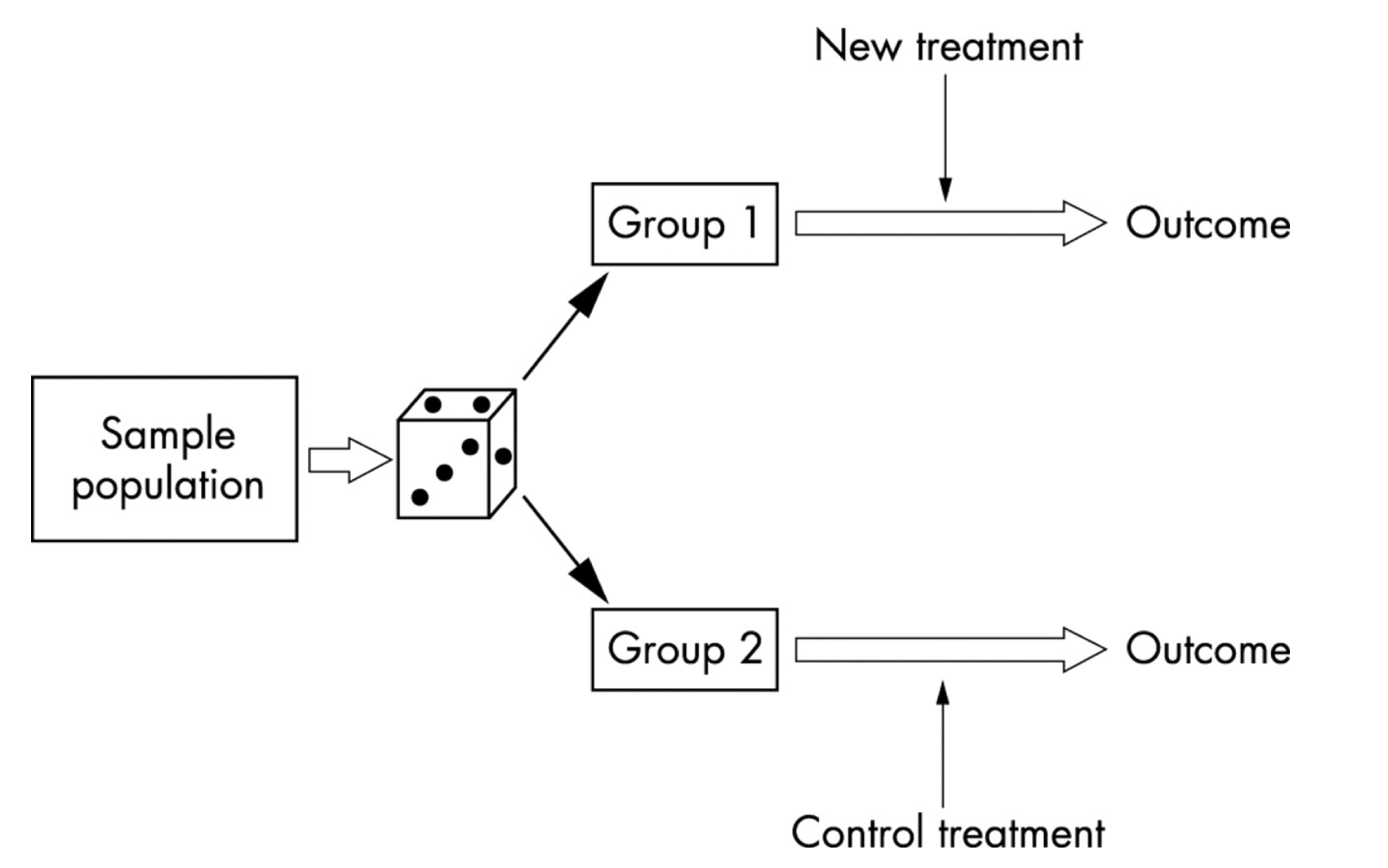
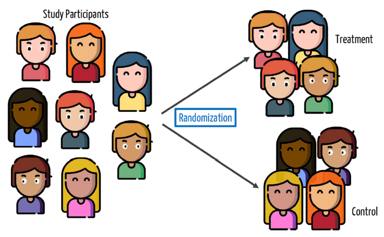
One way to make sure the causal conclusion holds is to do it by design:
Randomize the assignment of the treatment \(Z\)
i.e. Some units will randomly be chosen to be in the treatment group and others to be in the control group.
What does randomization buy us?
Control for unforeseen factors (confounders)
Confounders
- Confounder is a variable that affects both the treatment and the outcome
Randomization
- Due to randomization, we know that the treatment is not affected by a confounder
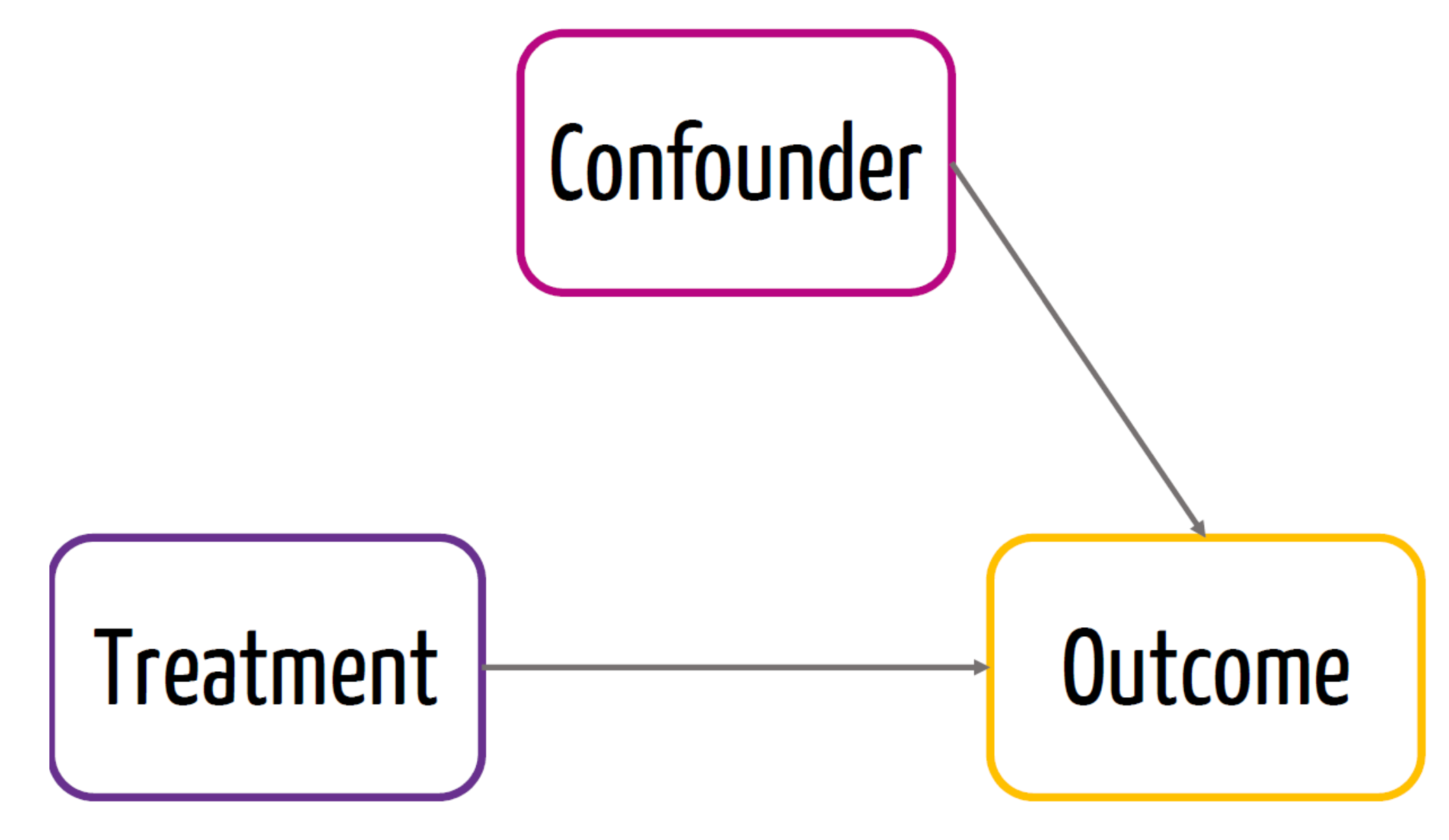
- This would be the causal effect of the treatment
Randomized controlled trials (RCTs)
Often called the gold standard for establishing causality.
Randomly assign the \(X\), treatment, to participants
Now, any observed relationship between \(X\) and \(Y\) must be due to \(X\), since the only reason an individual had a particular value of \(X\) was the random assignment.
Randomized controlled trials (RCTs)
RCT - Steps
Randomize
Check for balance - (balance between the treated and untreated)
Calculate difference in sample means between treatment and control group
Problem with causal inference
- Suppose you have a headache, and you take an asprin. Then you don’t have a headache. Did the asprin work?
| Person | Took aspirin | Didn’t take aspirin |
|---|---|---|
| 1 | no headache (0) | ? |
| 2 | no headache (0) | ? |
| 3 | no headache (0) | ? |
| 4 | no headache (0) | ? |
| 5 | ? | no headache (0) |
| 6 | ? | headache (1) |
| 7 | ? | headache (1) |
| 8 | ? | headache (1) |
- For any given person, we can only observe one outcome or the other, depending on whether the person took an asprin or not:
Problem with causal inference
The best we can do is compute an average treatment effect (ATE): the difference in the proportion of the treatment vs control group \[ \begin{aligned} \text{ATE} &= (\% \text{ headache among aspirin–takers}) \\ &\;\;-\; (\% \text{ headache among non–aspirin–takers}) \\ &= \frac{0}{4} - \frac{3}{4} \\ &= -0.75 \end{aligned} \]
Headaches decreased in 75% among those who took aspirin compared to those who didn’t take aspirin.
We can only make this conclusion if the treatment was randomly assigned.
Example 1: Vaccine Trial
Phase 3 Clinical Trial for the Moderna COVID-19 vaccine
\(X\) = got the vaccine, \(Y\) = got COVID-19
Randomly assign study participants to get either the vaccine (an treatment group of 14,134 people) or a placebo (a control group of 14,073 people)
11 vaccine recipients got COVID; 185 of placebo recipients got COVID
Issues with RCT
- Internal validity is the ability of an experiment to establish cause-and-effect of the treatment within the sample studied.
- Examples of threats to internal validity:
- Failure to randomize.
- Failure to follow the treatment protocol/attrition.
- Small sample sizes
Issues with RCT
- External validity is the ability of an experimental result to generalize to a larger context or population.
- Examples of threats to external validity:
- Non representative samples.
- Non representative protocol/policy.
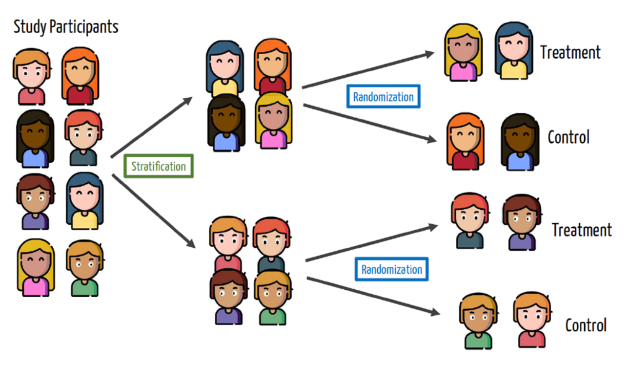
Blocking
Randomization works on average but we only get one opportunity at creating treatment and control groups, and there might be imbalances in nuisance variables that could affect the outcome.
For example, what will happen if the treatment group for the Moderna trial happens to get younger people in it than the control group?
We can solve this by blocking or stratifying: randomly assigning to treatment/control within groups.
Blocking
- Unbalanced sample - Males and Females
Blocking
- Blocking or stratification sample
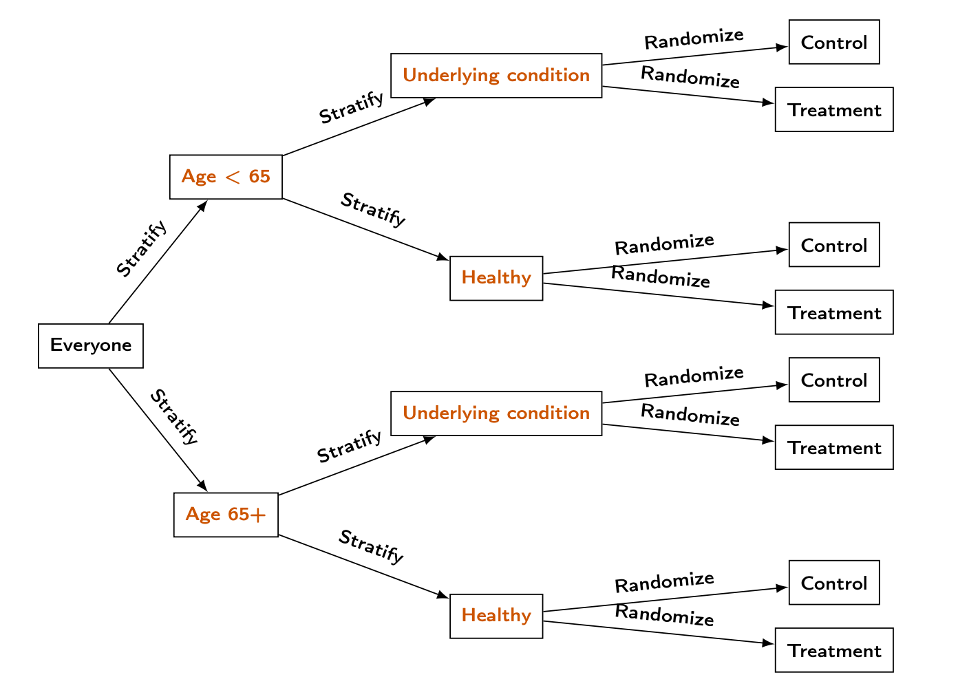
Blocking in vaccine trial
In the Moderna vaccine trial, they identified two possible variables that could impact COVID outcomes:
Age (65+ vs under 65)
Underlying health condition
Blocking in vaccine trial
Experiments using regression
Non-blocked design: use a simple regression \[ \widehat{Y} = \widehat{\beta}_0 + \widehat{\beta}_1 T, \]
where \(T\) is a dummy variable that is \[ T = \begin{cases} 1, & \text{for the treatment group}, \\ 0, & \text{for the control group} \end{cases} \]
\(\widehat{\beta}_1\) represents the estimated average treatment effect. With a binary \(Y\), ordinary least squares (a linear probability model) yields coefficients that are changes in the probability of \(Y=1\) (often reported as percentage points).
Experiments using regression
- Blocked design: use a regression that controls for the blocking variable \(B\):
\[ \widehat{Y} = \widehat{\beta}_0 + \widehat{\beta}_1 T + \widehat{\beta}_2 B, \] where \(B\) is the fixed effect of each strata, that are interactions between categories.
- Important: with a binary \(Y\), a linear probability model (OLS) is common; interpret slopes as percentage point changes in \(Y\).
Get Out The Vote (GOTV)
In 2002, researchers at Temple and Yale conducted a large phone banking experiment to see calling voters helps:
From among about 381,062 phone numbers of voters in Iowa and Michigan they randomly contacted about 12000 voters
The outcome Y of interest is whether each voter actually voted.
No blocking
Estimating the average treatment effect with a linear probability model (OLS):
- With a 0/1 outcome, OLS coefficients are changes in probability (multiply by 100 for percentage points).
No blocking
- The average treatment effect is the treatment coefficient on the probability scale: about 4.2 percentage points higher predicted turnout in the treatment group.
treatmenttreatment
        0.04191222
2.5 % 97.5 %
0.03286160 0.05096285 - Receiving a phone call is associated with about 4 percentage points higher predicted probability of voting than not receiving a call (linear probability model). The chunk above also prints the 95% CI for that effect in percentage points.
Blocking
The researchers actually used a blocking design with two variables that they thought could impact voting rates (separately from the phone calls):
The state of the voter (Iowa or Michigan)
Whether the voter was in a “competitive” district (one where there was likely to be a close election)
Blocking
Coding of state and competiv in GOTV.csv:
| Variable | Code | Meaning |
|---|---|---|
state |
0 | Michigan |
state |
1 | Iowa |
competiv |
1 | Less competitive district |
competiv |
2 | More competitive district |
Blocking

Blocking
Call:
lm(formula = vote02 ~ treatment + block, data = GOTV)

Residuals:
    Min      1Q  Median      3Q     Max
-0.6632 -0.5108  0.3437  0.4892  0.4892

Coefficients:
                   Estimate Std. Error t value            Pr(>|t|)
(Intercept)        0.510811   0.001026 498.075 <0.0000000000000002 ***
treatmenttreatment 0.006854   0.004670   1.468               0.142
block1.1           0.086655   0.003685  23.514 <0.0000000000000002 ***
block0.2           0.048892   0.002181  22.417 <0.0000000000000002 ***
block1.2           0.145496   0.002259  64.410 <0.0000000000000002 ***
---
Signif. codes:  0 '***' 0.001 '**' 0.01 '*' 0.05 '.' 0.1 ' ' 1

Residual standard error: 0.4948 on 381057 degrees of freedom
Multiple R-squared:  0.01166,   Adjusted R-squared:  0.01165
F-statistic:  1124 on 4 and 381057 DF,  p-value: < 0.00000000000000022
Blocking
- After controlling for block (
state\(\times\)competiv), the estimated treatment effect is only about 0.7 percentage points on the probability scale and is not statistically significant (linear probability model).
                          2.5 %     97.5 %
(Intercept)         0.508800670 0.51282084
treatmenttreatment -0.002299699 0.01600776
block1.1            0.079431705 0.09387772
block0.2            0.044617661 0.05316711
block1.2            0.141068386 0.14992313
What if some callers didn’t stick to the script?
Many people didn’t answer the phone!
What about voters outside of the Midwest?
The limitations of RCTs
Although powerful for inferring causation, RCTs are difficult to apply.
They can be incredibly expensive.
Compliance with the treatment protocol isn’t perfect (e.g., mask-wearing, picking up the phone)
It can be hard to generalize beyond the participants involved in the study.
They can be impractical or (e.g., effect of education on performance) or unethical to conduct (e.g., seatbelts, parachutes, even medical trials)
![]()