Data Science for Business Applications

Author

Class 01 - Linear Regression

Introduction

Course Goals

Use regression to build predictive models
Understand the benefits and limitations of the models we build
Given a new business situation, select an appropriate model, build it, measure its effectiveness, and effectively communicate the results
This is a practical course!

Why Does This Course Exist?

Why bother learning this stuff when we can get ChatGPT to do data analysis for us?
AI (and computing in general) is only useful when you have the expertise to be able to recognize the correctness (or not) of its output
In this class, you’ll develop that expertise!

About the Course Staff

Instructor: Henrique Bolfarine, Ph.D.
- Office hours: Mondays 1:00 PM - 2:00 PM (GSB 3.140 A)
- Email: henrique.bolfarine@austin.utexas.edu
Course Assistants:
- Lead Course Assistant (CA): Ezgi Durakoglugil
- Office hours: Many TA/CA office hours every week (both in person and on Zoom) - This should be your first option!
- You can ask any of the TAs/CAs about course content, but go to Ezgi for questions about logistics

Course logistics

Course Structure

Units
- Unit A: Fundamentals of regression modeling
- Unit B: Applications and extensions
Canvas
- Make sure you can log in and are enrolled in STA 235 in Canvas
- Check out the home page for the weekly schedule and to meet the course staff

Statistical Computing

We will use R and RStudio for statistical analysis throughout the course
Make sure both are installed on your laptop and bring it to every class
If you aren’t comfortable with R/RStudio from STA 301, don’t worry!

Weekly Cadence for a Particular Topic

Due by the start of class on Monday/Tuesday: Perusall pre-class video/reading discussion covering the topic
During class on Monday/Tuesday: Lecture, activities, practice topic
Due by 11:59 PM the following Sunday/Monday: Homework covering the topic
The following Monday/Tuesday: at the beginning of class: Checkpoint Quiz on that topic

Pre-Class Work

This is a fast-paced course, so it’s essential that you think about the material before class.
We will use Perusall for pre-class video and reading assignments.
Use Perusall to ask your classmates questions, and share your knowledge, thoughts, and opinions.
This helps you better understand the material and will help me gear class time to what topics you are having the most trouble with.

Pre-Class Work

Pre-class assignments (typically videos) are due at the start of each class.
Aim to chime in with at least a few thoughtful questions, responses, or comments for each reading assignment.
Grading is based on effort and thoughtfulness of your questions and comments and your engagement with classmates and the text.
Each assignment is scored 0-3, but with a reasonable effort you will get a 3 on each one (so don’t worry about your grade).

Homework

Why homework?
Homework is due each week at 11:59 PM the night before class and submitted through Canvas.
Automatically graded; resubmit as many times as you want!
OK to work together, but try the problems on your own first for maximum benefit.

Checkpoint Quizzes

It is critical in this course to stay on top of things and not fall behind.
Checkpoint Quiz at the start of each class will help you ensure that you are really learning the material and give you an early heads-up if you aren’t.
We’ll drop your lowest quiz score from each unit (A and B).
You’ll have access to RStudio and a “cheat sheet” during quizzes (don’t spend time memorizing anything!).

Mastery Exams

Each unit concludes with a Mastery Exam:
- Unit A: October 22 or 23 at 7 to 9 PM
- Unit B: University-assigned final exam period
You’ll have access to RStudio and a “cheat sheet” during exams (don’t spend time memorizing anything!).

Assessment Grading

Unit A has 7 Checkpoint Quizzes and Unit B has 6.
For each unit, we will replace your lowest quiz score with your exam score for that unit (if that helps your overall grade).

Grading

Component	Points
Pre-class work (Perusall)	44
Class Participation	56
Homework (13)	195
Checkpoint Quizze (13)	325
Exam A	190
Exam B	190
Total	1,000

Getting Help

My office hours: Schedule on Canvas.
TA/CA office hours: Schedule on Canvas.
Post questions in videos in Perusall (for questions about the course material).
Post questions in group chats in Perusall (for general questions about the course, or homework questions).
Weekly optional TA/CA-led review session (TBD).

Simple Regression

What personal characteristics about an instructor do you think are predictive of the scores they receive on student evaluations?

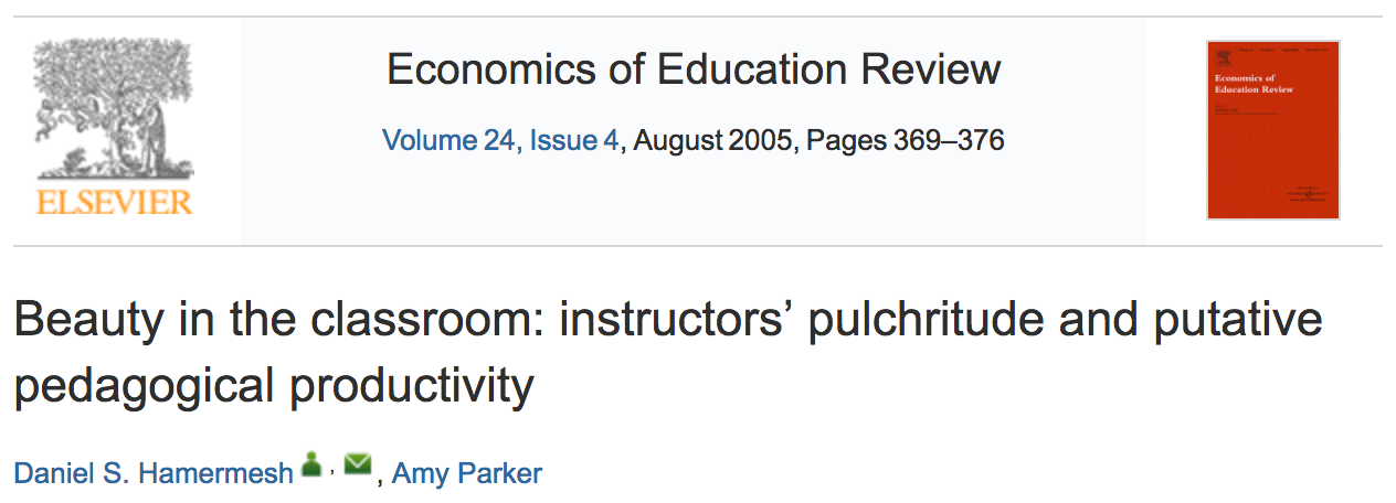
Hamermesh & Parker (2005) Data Set

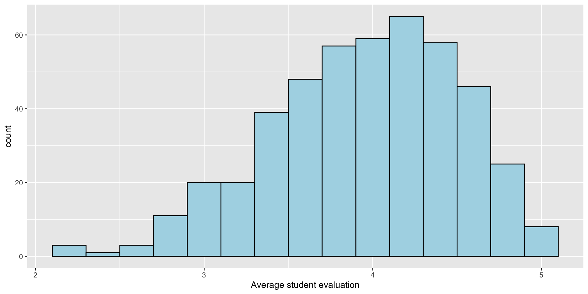
Student evaluations of $N=463$ instructors at UT Austin, 2000-2002
For each instructor:
eval: average student evaluation of teacher
beauty: average beauty score from a six-student panel
gender: male or female
credits: single- or multi-credit course
age: age of instructor
(and more…)

Explore the data: `eval`

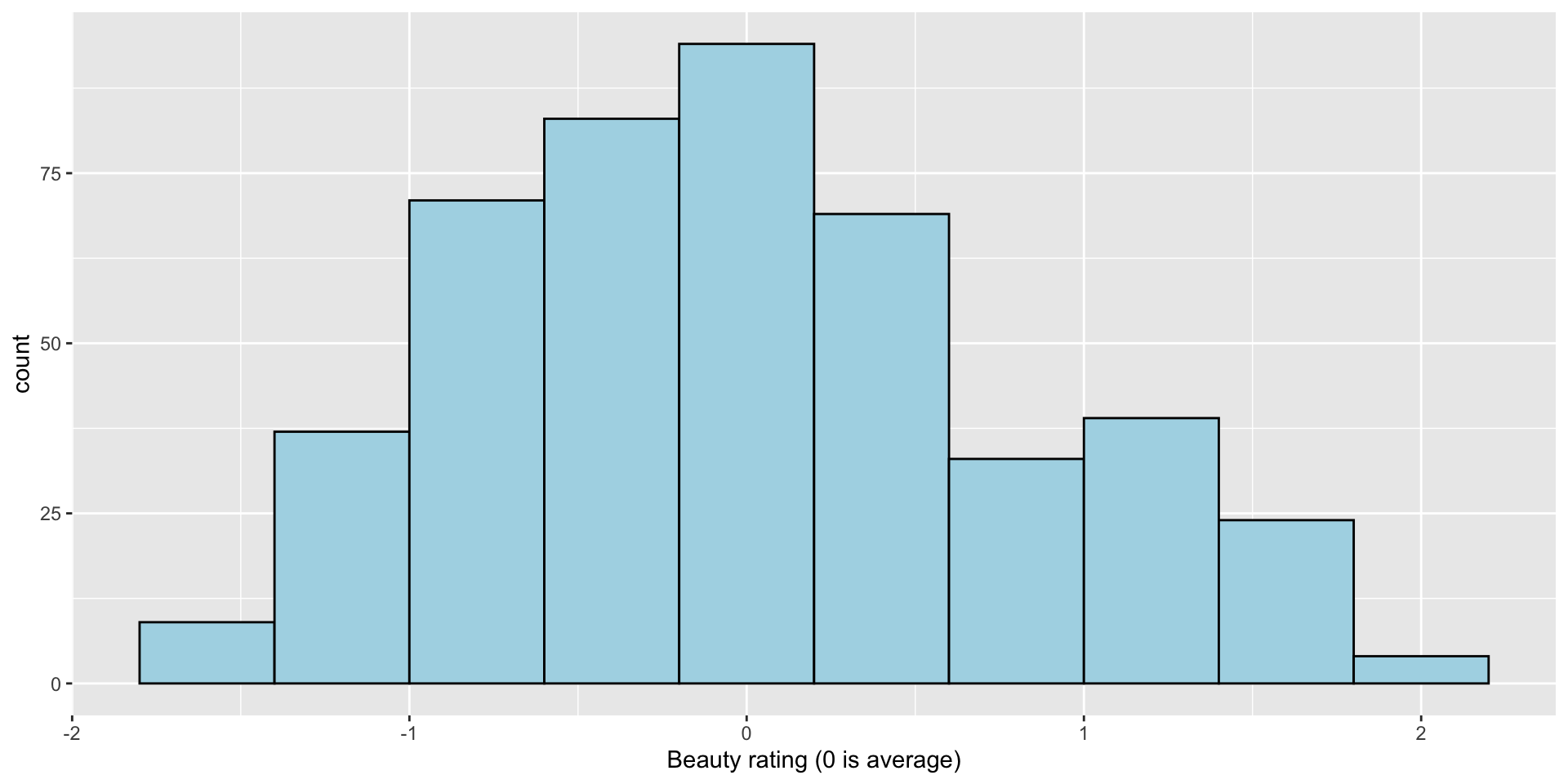
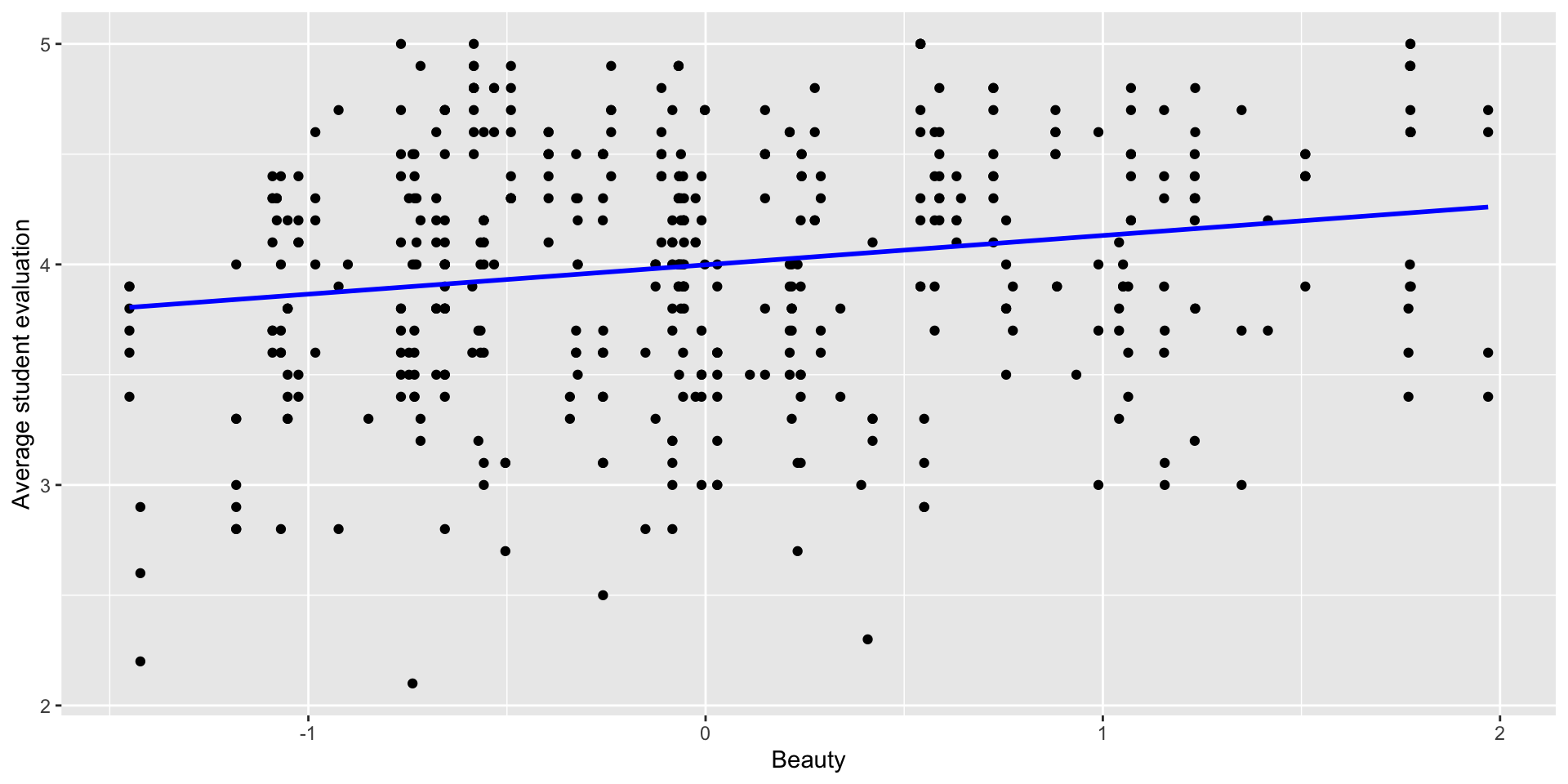
Explore the data: `beauty`

Explore the data

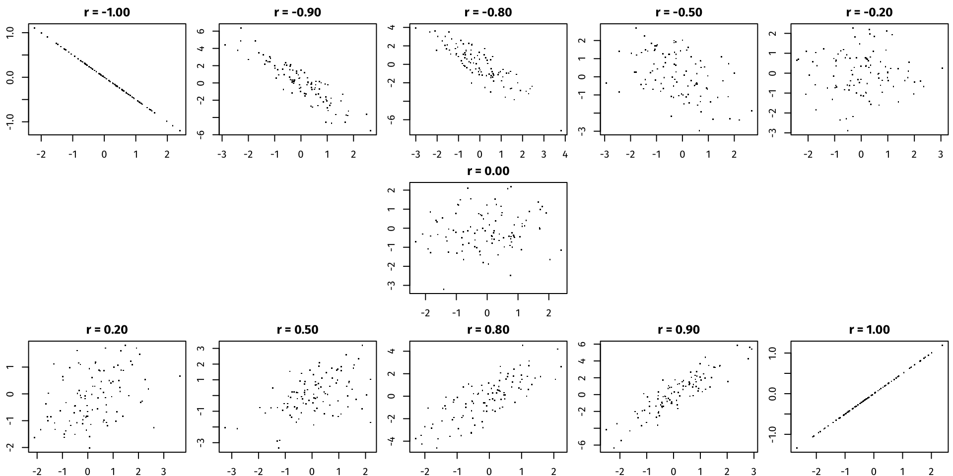
Correlation

The correlation $r$ between two variables $X$ and $Y$ measures the strength of the linear relationship between them. Correlation ranges from $-1$ (perfect negative relationship) to $0$ (no relationship) to $1$ (perfect positive relationship).

Correlation

Correlation

cor(profs$eval, profs$beauty)

[1] 0.1890391

How can we interpret this?
The $ sign accesses the variables in the data set profs.csv.

Let’s Build a Simple Regression Model

\[ \text{eval} = \beta_0 + \beta_1 \cdot \text{beauty} + \epsilon \]

$\beta_0$ and $\beta_1$ are known as coefficients (standard notations)
$\beta_0$ is the intercept
$\beta_1$ is the slope associated with beauty
The term $\epsilon$ (epsilon) accounts for unobserved factors that are not included in this model

Let’s Build a Simple Regression Model in Rstudio

# Build a simple regression model
model <- lm(eval ~ beauty, data = profs)
summary(model)


Call:
lm(formula = eval ~ beauty, data = profs)

Residuals:
     Min       1Q   Median       3Q      Max 
-1.80015 -0.36304  0.07254  0.40207  1.10373 

Coefficients:
            Estimate Std. Error t value             Pr(>|t|)    
(Intercept)  3.99827    0.02535 157.727 < 0.0000000000000002 ***
beauty       0.13300    0.03218   4.133            0.0000425 ***
---
Signif. codes:  0 '***' 0.001 '**' 0.01 '*' 0.05 '.' 0.1 ' ' 1

Residual standard error: 0.5455 on 461 degrees of freedom
Multiple R-squared:  0.03574,   Adjusted R-squared:  0.03364 
F-statistic: 17.08 on 1 and 461 DF,  p-value: 0.00004247

Interpreting the Model

eval is the response variable ($Y$); beauty is the predictor variable ($X$).
Simple regression uses the best fit line to give us a linear equation to predict $Y$ from $X$:

\[ \widehat{\text{eval}} = 3.998 + 0.133 \cdot \text{beauty} \]
We can predict the evaluation score for someone based on their beauty score just by plugging into the equation.
What do the coefficients mean?

Interpretation

Intercept
- When the beauty score is zero, the expected evaluation is 3.99 (almost 4).
- Here, beauty = 0 represents an “average beauty”.
- Important, the intercept is evaluated always when the predictor variable is zero.
Slope for Beauty
- For every one-unit increase in the beauty score, there is a 0.133 increase in the professor’s expected evaluation.
- In this context, “expected” refers to the average evaluation.

Statistical Significance of the Model

The population regression line (the best fit line in the population) is $Y = \beta_0 + \beta_1 X$ (we can’t know this).
Our regression equation is the best fit line in the sample, or $\hat{Y} = \hat{\beta}_0 + \hat{\beta}_1 X$ (this is what we get from our sample data).
The sample intercept and slope $\hat{\beta}_0$ and $\hat{\beta}_1$ are our best estimates for the population intercept and slope $\beta_0$ and $\beta_1$.
But we need to get a sense of how close $\hat{\beta}_0$ and $\hat{\beta}_1$ are to $\beta_0$ and $\beta_1$!

P-values

For this model, the p-values associated with the coefficients, slope and intercept are close to zero:

Term	p-value - `Pr(>\|t\|)`	Significance
Intercept	0.0000000000000002	***
Beauty	0.0000425	***

In this case, there’s evidence that beauty has an impact on a professor’s evaluation at a populational level.
Thus, we can conclude that the effect of beauty is statistically significant in relation to the professor’s evaluation.

Rule of Thumb for P-values

If the p-value is smaller than 0.05, we can conclude that the effect is statistically significant.
Otherwise, if the p-value is greater than 0.05, we conclude that the effect from the predictor is not statistically significant.

Confidence Intervals

Let’s get confidence intervals for the slope and intercept to get a sense of the uncertainty in our estimates:

confint(model)

                 2.5 %    97.5 %
(Intercept) 3.94845765 4.0480866
beauty      0.06976869 0.1962342

Slope: We are 95% confident that the incremental impact of each additional beauty point is between $0.07$ and $0.20$ student evaluation points.
Intercept: We are 95% confident that the average student evaluation score for average-looking professors (beauty = 0) is between $3.95$ and $4.05$.
Rule of thumb: If zero is inside the CI, the effect is not statistically significant.
P-values and confidence intervals (CIs) are connected. If the p-value is greater than 0.05, it is likely that zero will be included within the confidence interval.

Confidence intervals for predictions

Interval for a single prediction:
- We are 95% confident that a single professor with a beauty score of 1 will get rated between 3.06 and 5.21.
```
predict(model, list(beauty=1), interval="prediction")
```
```
       fit      lwr      upr
1 4.131274 3.056375 5.206172
```
Interval for an average prediction:
- We are 95% confident that the average rating of all professors with beauty scores of 1 will be between 4.05 and 4.21.
```
predict(model, list(beauty=1), interval="confidence")
```
```
       fit      lwr      upr
1 4.131274 4.050776 4.211771
```

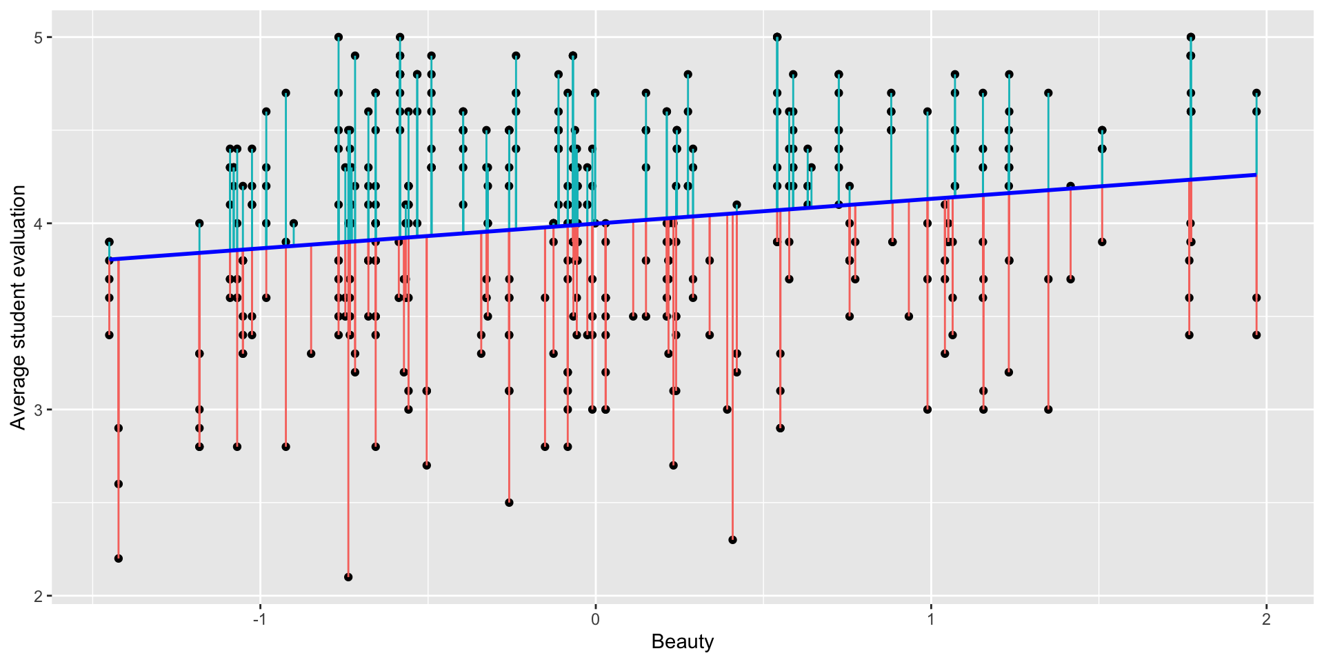
Residuals and R-squared

Each instructor has a residual: the difference between their actual and predicted scores (the prediction error).

Residual standard error

The residual standard error is in the same units as the response variable:
- In this case the RSE is: Residual standard error: 0.5455
- All predictions made by this model will, on average, differ from the true values by approximately 0.5455, which represents one standard deviation of the residuals.
We can even get the 95% prediction interval for a single (beauty = 1) prediction as
- lower bound: $3.998 + 0.133 \cdot 1 - 2\times \text{RSE}$
- upper bound: $3.998 + 0.133 \cdot 1 + 2\times \text{RSE}$

# lower bound 
3.998 + 0.133 - 2*0.5455

[1] 3.04

# upper bound
3.998 + 0.133 + 2*0.5455

[1] 5.222

R-squared ($R^2$)

The $R^2$ provides an understanding of the “fit” of the model in relation to the data.
- If the $R^2$ is close to one, the model has a good fit.
- If the $R^2$ is close to zero, the model does not provide a good fit for the data.
- Multiple R-squared: 0.03574
- This indicates not a great fit.
Important interpretation:
- The $R^2$ represents the percentage of variation in the response variable that can be explained by the predictor.
- For this model, 3.6% of the variation in evaluation scores can be explained by the beauty variable alone, while the remaining 96.4% is attributed to other unobserved factors.

Multiple Regression

Adding more predictors

Is the professor’s evaluation explained only by it’s beauty or there might be other factor affecting their evalution?
Let’s check if the variable age might help us better explain the relationship between beauty and evaluation.
We update our model as:

\[ \widehat{\text{eval}} = \beta_0 + \beta_1 \cdot \text{beauty} + \beta_2 \cdot \text{age} + \epsilon \] - We now have a multiple regression model. - Both beauty and age are numerical variables. - The term $\epsilon$ (epsilon) accounts for unobserved factors that are not included in this model.

Multiple regression model

# Build a simple regression model
model <- lm(eval ~ beauty + age, data = profs)
summary(model)


Call:
lm(formula = eval ~ beauty + age, data = profs)

Residuals:
     Min       1Q   Median       3Q      Max 
-1.80242 -0.36514  0.07407  0.39913  1.10206 

Coefficients:
             Estimate Std. Error t value             Pr(>|t|)    
(Intercept) 3.9844013  0.1337296  29.794 < 0.0000000000000002 ***
beauty      0.1340634  0.0337441   3.973            0.0000824 ***
age         0.0002868  0.0027148   0.106                0.916    
---
Signif. codes:  0 '***' 0.001 '**' 0.01 '*' 0.05 '.' 0.1 ' ' 1

Residual standard error: 0.546 on 460 degrees of freedom
Multiple R-squared:  0.03576,   Adjusted R-squared:  0.03157 
F-statistic:  8.53 on 2 and 460 DF,  p-value: 0.0002305

How can we interpret this model?

Interpretation of Model Coefficients

Intercept
- When both the beauty score and age are zero, the expected evaluation is 3.98 (almost 4).
- Here, beauty = 0 represents an “average beauty,” and age = 0 is not meaningful in this context but is part of the model.
- Important: The intercept is evaluated when all predictor variables (beauty and age) are zero.
Slope for Beauty
- For every one-unit increase in the beauty score, there is a 0.134 increase in the professor’s expected evaluation, holding age constant.
Slope for Age
- For every one-unit increase in age, there is a 0.0003 increase in the professor’s expected evaluation, holding beauty constant.

Statistical significance

For this model, the p-values associated with the coefficients (intercept, beauty, and age) are as follows:

Term	p-value - `Pr(>\|t\|)`	Significance
Intercept	< 0.0000000000000002	***
Beauty	0.0000824	***
Age	0.916

In this model, there is strong evidence that beauty has an impact on a professor’s evaluation at the population level, as its p-value is very close to zero.
However, the p-value for age (0.916 > 0.05) indicates that there is no statistically significant relationship between age and a professor’s evaluation.
Thus, we can conclude that the effect of beauty is statistically significant in relation to a professor’s evaluation, while the effect of age is not statistically significant.

RSE and $R^2$

There are no significant changes in relation to the RSE and $R^2$ in relation to the previous model.
This means that the quality of the fit and the accuracy of the predictions will be nearly identical to those of the previous model.
For this model, 3.6% of the variation in evaluation scores can be explained by the beauty and age variables alone, while the remaining 96.4% is attributed to other unobserved factors.
What about predictions and confidence intervals?

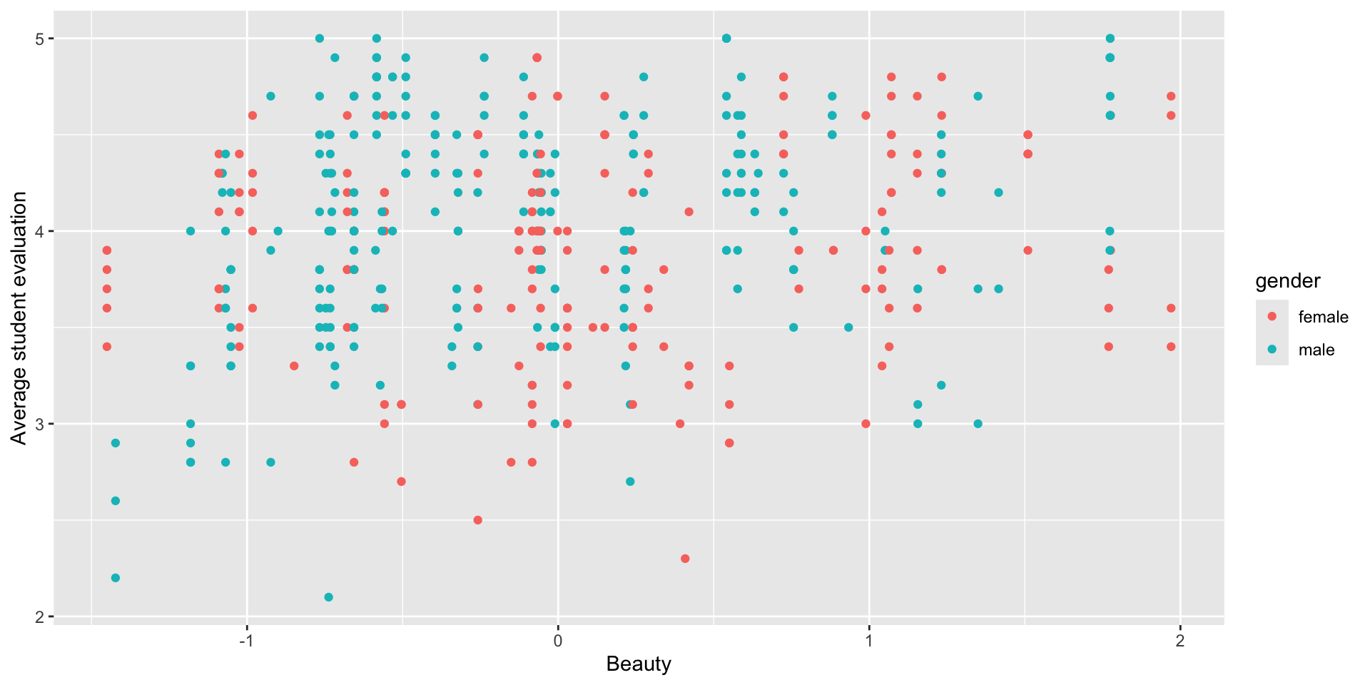
What’s the Impact of Gender on Student Evaluations?

Do you see a difference between men (blue) and women (red)?

For for the Weekend

Read the syllabus.
Do the first homework assignment in Canvas (covering today’s material).
Do the first pre-class assignment in Perusall (to prepare for next week’s class).

Other Formats

Introduction

Course Goals

Why Does This Course Exist?

About the Course Staff

Course logistics

Course Structure

Statistical Computing

Weekly Cadence for a Particular Topic

Pre-Class Work

Pre-Class Work

Homework

Checkpoint Quizzes

Mastery Exams

Assessment Grading

Grading

Getting Help

Simple Regression

Hamermesh & Parker (2005) Data Set

Explore the data: eval

Explore the data: beauty

Explore the data

Correlation

Correlation

Correlation

Let’s Build a Simple Regression Model

Let’s Build a Simple Regression Model in Rstudio

Interpreting the Model

Interpretation

Statistical Significance of the Model

P-values

Rule of Thumb for P-values

Confidence Intervals

Confidence intervals for predictions

Residuals and R-squared

Residual standard error

R-squared (\(R^2\))

Multiple Regression

Adding more predictors

Multiple regression model

Interpretation of Model Coefficients

Statistical significance

RSE and \(R^2\)

What’s the Impact of Gender on Student Evaluations?

For for the Weekend

Explore the data: `eval`

Explore the data: `beauty`