Data Science for Business Applications

Author

Class 10 - Decision Trees

Decision Trees

Another predictive model
Decision Trees: Classification and Regression Trees (CART)
Trees are:
- Flexible at capturing non-linearity and interactions
- Don’t require scaling of variables
- Handle categorical and numerical data
- Fast
- Interpretable

The Idea Behind Decision Trees

Create a flow chart for making decisions
- How do we classify an individual?
But there are many decisions!
- How many variables do we use?
- How do we sort them? In what order do we place them?
- How do we split them?
- How deep do we go?

The Idea Behind Decision Trees

The decision tree is always binary
Splits the data in two parts given a decision rule
Structure:
- Root node (decision rule)
- Internal nodes (decision rule)
- Leaves (prediction)

Types of Decision Tree

We can use decision trees to perform:
- Classification tasks (target variable is categorical)
  - Similar to logistic regression
- Regression (target variable is numerical)
  - Works well on nonlinear data

Creating a Decision Tree

Determine which variable and criteria we can use to split the data into two groups (binary) so that the two parts of the data are as different as possible from each other
Within each group, repeat step 1
Stop this process when we run out of variables, or splitting no longer helps us make better predictions

Creating a Decision Tree (Basically)

Start at the root node
Split by a variable that provides the most differentiation
Stop splitting if you get pure leaves or pure enough (one class)
Repeat for each node
Assign the majority classification (or average outcome in regression)

Example - Disney+

Disney+ data:
- city: Whether the customer lives in a big city or not
- female: Whether the customer is female or not
- age: Customer’s age (in years)
- logins: Number of logins to the platform in the past week
- mandalorian: Whether the person has watched the Mandalorian or not
- unsubscribe: Whether they canceled their subscription or not
Let’s try to predict who will cancel their subscription

Predicting subscription

Since our outcome is binary, this is a classification task
We’ll start with two variables, city and mandalorian
Here’s a frequency table:

unsub_df = disney %>%
  filter(unsubscribe == "unsubscribe")

xtabs(~mandalorian + city, data = unsub_df) %>% 
  addmargins()

           city
mandalorian   no  yes  Sum
        no    22  152  174
        yes  183  995 1178
        Sum  205 1147 1352

stay_df = disney %>%
  filter(unsubscribe == "stay")

xtabs(~mandalorian + city, data = stay_df) %>% 
  addmargins()

           city
mandalorian   no  yes  Sum
        no   190 1101 1291
        yes  317 2040 2357
        Sum  507 3141 3648

For mandalorian:

Mandalorian	Subscribers	Unsubscribers	Total	% Unsubscribed
no	1291	174	1465	11.9%
yes	2357	1178	3535	33.3%

There’s a big difference in unsubscribe rates between those who watched and didn’t watch The Mandalorian.
This suggests mandalorian is a strong predictor of unsubscribe.
For city:

City	Subscribers	Unsubscribers	Total	% Unsubscribed
no	507	205	712	28.8%
yes	3141	1147	4288	26.7%

There’s also a difference, but it’s smaller than for mandalorian.

The variable that most reduces impurity, that makes each resulting group more “pure” in terms of unsubscribe/stay gets chosen for the first split in this case mandalorian.

We can then classify based on the majority percentage in each leaf node
In this case very intersting sincethe prediction will always be subscribe

Adding `city`

Let’s add city in both nodes

City	Type	Mandalorian `No`	Mandalorian `Yes`
`No`	Unsubscribers	22	183
`No`	Subscribers	190	317
`Yes`	Unsubscribers	152	995
`Yes`	Subscribers	1101	2040

Results in the follwing tree

This tree is not really good since it always predict subscription.

Example with data

Can We Build a Model to Predict Who Survived the Titanic?
We’ll make a classification tree to predict survival:
- adult: If the passenger was as or older than 18
- sex: passenger’s gender; male or female
- passengerClass: Class in which the passenger traveled: 1st, 2nd, 3rd
- survided: Indicates if the passenger survived or not: yes, no

Build the tree

Before we can build the tree we should define the categorical variables as factors.
This is not necessary when the variables are binary or dummy (0 or 1).

library(tidyverse)
library(tidymodels)
library(rpart.plot)

titanic_age$survived = as.factor(titanic_age$survived)
titanic_age$sex = as.factor(titanic_age$sex)
titanic_age$passengerClass = as.factor(titanic_age$passengerClass)
titanic_age$adult = as.factor(titanic_age$adult)

Build the tree

# Create a decision tree model specification
tree_spec <- decision_tree(mode = "classification",engine = "rpart")

# Fit the model to the training data
tree_fit <- tree_spec %>%
  fit(survived ~ adult + sex + passengerClass, data = titanic_age)

### Model Results
# Print out the logic the decision tree decided on
rules <- rpart.rules(tree_fit$fit)
print(rules)

 survived                                                  
     0.21 when sex is   male                               
     0.47 when sex is female & passengerClass is        3rd
     0.93 when sex is female & passengerClass is 1st or 2nd

This decision tree shows us that:
- 0.21, or 21%, of the men on the Titanic survived
- 0.47, or 47%, of the females in the third class survived
- 0.93, or 93%, of the females in the 1st or 2nd survived
In some ways the tree returns the probability of surviving given the conditions displayed on the decision rules.

Plot the decision rules and classification

# Plot the decision tree
rpart.plot(tree_fit$fit, type = 4, extra = 101, 
           under = TRUE, cex = 0.8, box.palette = "auto")

How to interpret the tree

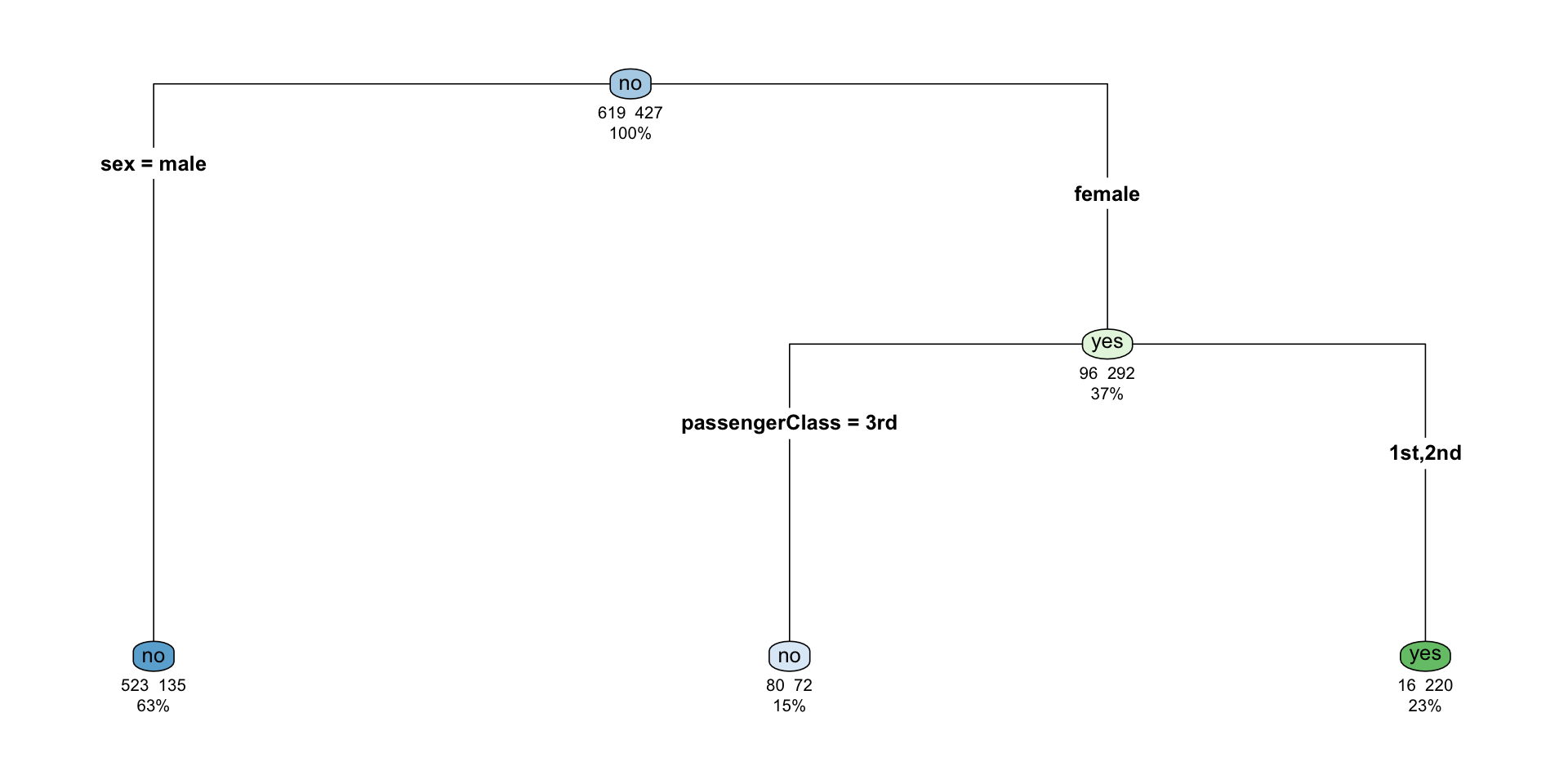
The nodes indicates which group of the target variable is more common in the split. If it indicates no it means that there’s a higher chance of not surviving than surviving.
So in the top node we have no and it indicates that from a total of 1046 (100%), 619 survived, and 427 did not.
We then use the first decision rule that splits the data into gender. It indicates that 63% (658) of the passengers are male and 37% (388) female. From those who are male, 523 died and 135 survived; that is 135/658 = 0.21, or 21%. In this case 523/658 = 0.79, or 79%, died. That’s the reason the node is no on the node.
From the 388 females, 152 were in the 3rd class, from which 80/152 = 0.53, or 53%, died, and 72/152 = 0.47, or 47%, survived. Of the female passengers in the 3rd class, 16/236 = 0.067, or 6.7%, died, and 220/236 = 0.93, or 93%, survived. In this case we can see that the node indicates an yes.
Overall the female node indicates that 96/388 = 24% of the female passengers died and 292/388 = 75% survived.

Using the model to make predictions

# Make predictions on the testing data
predictions <- tree_fit %>%
  predict(titanic_age) %>%
  pull(.pred_class)

titanic_age = titanic_age %>% 
  mutate(pred.survival = predictions)

xtabs(~pred.survival+survived,data=titanic_age) %>% 
  addmargins()

             survived
pred.survival   no  yes  Sum
          no   603  207  810
          yes   16  220  236
          Sum  619  427 1046

Since this is classification model we can measure the accuracy of the model
- True positives (TP) - 220
- True Negatives (TN) - 603
- False Positives (FP) - 16
- False Negatives (FN) - 207
Accuracy is equal to (TP+TN)/Total = (220+603)/1046 = 0.78, or 78%

Regression Trees

We can also use decision trees for regression.
We’ll use our Boston data for predicting median home value (MEDV), measured in thousands of dollars, from a socioeconomic indicator LSTAT that was defined as the proportion of adults without some high school education and proportion of male workers classified as laborers). There are 506 observations in this data.
In this case, both the target variable and the predictor are numerical, and the nodes will show the average value of this variable (average of the median home value).
The decision on the node (rule) of the tree will now depend on a numerical cutoff determined by the data, which will split the predictor into areas from which a prediction will be made by obtaining the average of the response in this area.

Running the model

# Make predictions on the testing data
# Create a decision tree model specification
tree_spec <- decision_tree(mode = "regression",engine = "rpart")

# Fit the model to the training data
tree_fit <- tree_spec %>%
  fit(MEDV ~ LSTAT, data = tree_housing)

Regression tree plot

rpart.plot(tree_fit$fit, type = 4, extra = 101, 
           under = TRUE, cex = 0.8, box.palette = "auto")

Regression tree interpretation

We start at the top, or root node of the tree. At each interior node we have a rule that tells us which split to take, based on the value of our predictor variable and the cutoff.
We keep going until we reach the bottom, or leaf node.
Within each partition, the target values are averaged to give us the prediction within that partition. These are also the values seen at the leaf nodes on the left
To predict a new point, we can just “drop” an observation down the tree until we end up at a leaf node.

Regression tree model

What does the regression tree look like applied to the data?
It is basically a step function in which the splits are determined by the tree structure.

How we evaluate the regression tree

We can also split the data into testing and training, or use cross validation and obtain the RMSE.
In this case we’ll only obtain the RMSE and the R-squared of this model on the original data as

# Make predictions on the testing data
predictions <- tree_fit %>%
  predict(tree_housing) %>%
  pull(.pred)

# Calculate RMSE and R-squared
metrics <- metric_set(rmse, rsq)
model_performance <- tree_housing %>%
  mutate(predictions = predictions) %>%
  metrics(truth = MEDV, estimate = predictions)

print(model_performance)

# A tibble: 2 × 3
  .metric .estimator .estimate
  <chr>   <chr>          <dbl>
1 rmse    standard       5.07 
2 rsq     standard       0.695

Model Results

Our median home estimates will have a prediction error of +/- 5.071 thousand dollars.
Our model captures 69.5% of the variation in age using the LSTAT variable.

More predictors on the regression tree

What if we had a tree with more than one explanatory variable?
We add distance to employment centers (DIS) to our model, and the tree can now use either LSTAT or DIS.

# Make predictions on the testing data
# Create a decision tree model specification
tree_spec <- decision_tree(mode = "regression",engine = "rpart")

# Fit the model to the training data
tree_fit <- tree_spec %>%
  fit(MEDV ~ LSTAT + as.numeric(DIS), data = tree_housing)

Regression tree plot

rpart.plot(tree_fit$fit, type = 4, extra = 101, 
           under = TRUE, cex = 0.8, box.palette = "auto")

Model performance

# Make predictions on the testing data
predictions <- tree_fit %>%
  predict(tree_housing) %>%
  pull(.pred)

# Calculate RMSE and R-squared
metrics <- metric_set(rmse, rsq)
model_performance <- tree_housing %>%
  mutate(predictions = predictions) %>%
  metrics(truth = MEDV, estimate = predictions)

print(model_performance)

# A tibble: 2 × 3
  .metric .estimator .estimate
  <chr>   <chr>          <dbl>
1 rmse    standard       4.85 
2 rsq     standard       0.721

In this case there is a slight increase in the R-squared and an increase in the RMSE, indicating a better fit compared to the previous model.

When to use decision trees?

Main Advantages:
- Easy to interpret and explain (you can plot them!)
- Mirrors human decision-making
- Can handle qualitative predictors (without need for dummies)
Main disadvantages:
- Accuracy not as high as other methods
- Very sensitive to training data (e.g. overfitting)

Other Formats

Decision Trees

The Idea Behind Decision Trees

The Idea Behind Decision Trees

Types of Decision Tree

Creating a Decision Tree

Creating a Decision Tree (Basically)

Example - Disney+

Predicting subscription

Adding city

Results in the follwing tree

Example with data

Build the tree

Build the tree

Plot the decision rules and classification

How to interpret the tree

Using the model to make predictions

Regression Trees

Running the model

Regression tree plot

Regression tree interpretation

Regression tree model

How we evaluate the regression tree

Model Results

More predictors on the regression tree

Regression tree plot

Model performance

When to use decision trees?

Adding `city`